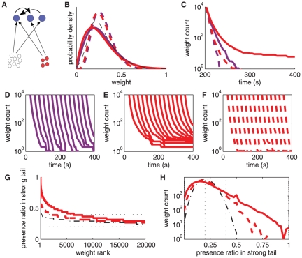
Figure 9. Stability of the emerging structure of strong weights in a recurrently connected network.
A: Schematic representation of the network with plastic recurrent connections (thick arrows) and fixed input connections (thin arrows). The network neurons (top blue filled circles) are excited by one pool of 2900 uncorrelated inputs (bottom open circles), and one pool of 100 inputs (bottom red filled circles) whose spike trains may be correlated. B: Time-averaged distributions of the recurrent weights over the learning epoch. Comparison of log-STDP (solid curves) and mlt-STDP (dashed curves) when the small group (red filled circles in A) is uncorrelated (purple) and correlated (red). C: Survival of strong synapses (top 20%) of the distribution over time. The color coding is similar to B. As in Fig. 5C, checks are performed every 5 s and the y-axis indicates the number of surviving synapses from  s until the time on the x-axis, cf. (8). D,E,F: Similar curves to B with different starting times
  . Comparison of D log-STDP with no correlation; E log-STDP with correlations; and F mlt-STDP with correlations. G: Ratio of presence in the top 20% at each check (every 5 s between 200 and 395 s) for the initially strongest at
  s, cf. (9). Comparison between log-STDP (solid curve) and mlt-STDP (dashed curve) for correlated inputs. The weight indices (x-axis) are sorted. The two horizontal dotted lines indicate 20% and 40%, respectively. H: Distributions of the presence ratio corresponding to G, with a log-scaled y-axis.

