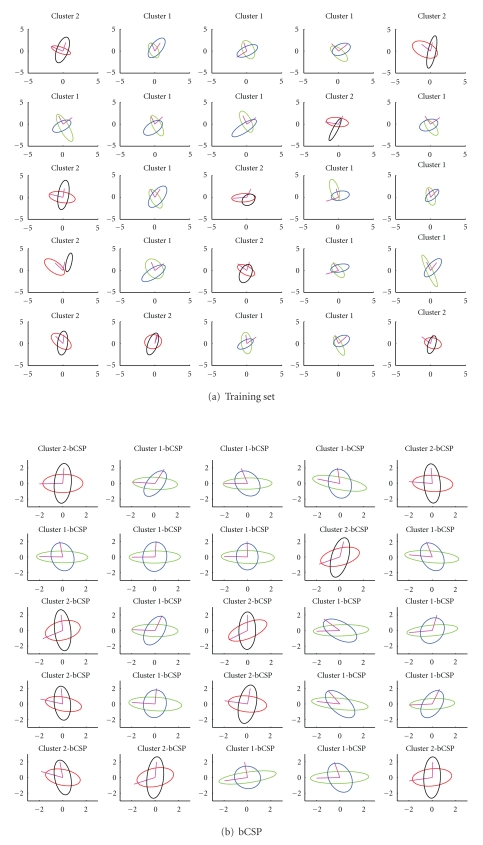
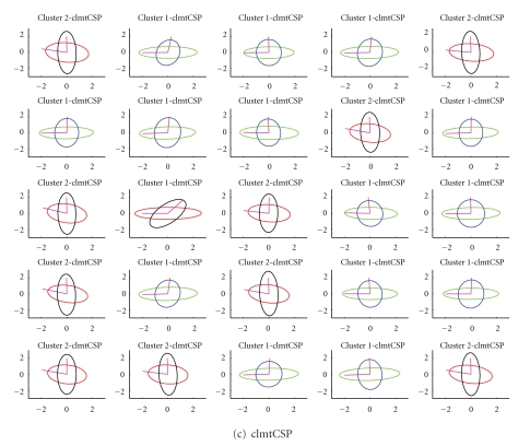
Figure 1.
(a) shows the training set that is used to compute both the bCSP and clmtCSP filters. The data points themselves are not plotted, instead we only draw the standard deviation contours of the data's estimated covariance matrix, together with its corresponding principal vectors (representing the ellipse's principal axis). Blue and black contours correspond to the first class or condition, while green and red contours represent the other class. The goal of the computed filters is to align the principal vectors to the axes. The results for both bCSP and clmtCSP are shown in (b) and (c) figures, respectively. Here, the contours denote the standard deviations according to the estimated covariance matrix of the “unmixed” sources. Concerning the clmtCSP method, if the contours are drawn in blue and green, it means that they have been estimated as being in the first cluster according to the algorithm. If it is red and black, the task is estimated as belonging to the second cluster. The true cluster number is given in the title of each subplot.


