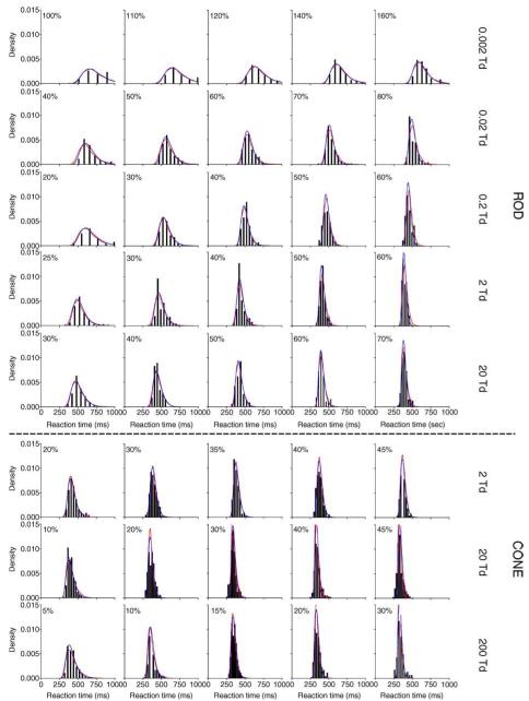
Figure 3.

The RT distributions for rod incremental stimuli at 0.002–20 Td (top 5 rows) and cone stimuli at 2–200 Td (bottom 3 rows) for observer DC. Each row represents data at one retinal illuminance level as labeled on the right. Each panel shows the RT distribution at one Weber contrast, as labeled within the panel. The separation between bars for the histograms indicates the optical bar width for distribution fitting using the method described by Scott (1979). The fitted probability density functions by the IRF-based model and the EZ diffusion model are shown as red and blue lines in each panel, respectively. Both models fit the RT distributions equally well.