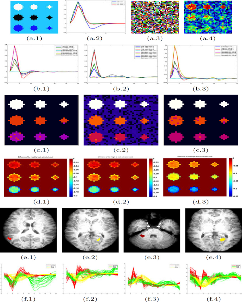
Fig. 1.
Set-up of Simulation: (a.1) a temporal cut of the true images; (a.2) the true curves of HRF: h1(t), h2(t) and h3(t); (a.3) a temporal cut of the simulated images; (a.4) the Gaussian smooth result. The estimated results: estimates of HRF for the (b.1 and c.1) 1st; (b.2 and c.2) 2nd; (b.3 and c.3) 3rd sequence of events. The row (b.1–3) is the average estimated HRF in each cluster. The row (c.1–3) is the recovered pattern relative to each sequence of events. The comparison statistics Dj with sFIR: (d.1–3) the difference of estimated Height(H) at each voxel for the three stimulus sequences. The color bar denotes the value of Dj for the jth voxel. Data analysis results: (e.1)–(e.4) the slices containing ROIs (colored ones) of the F maps for the 1st–4th stimulus sequences, respectively; (f.1)–(f.4) estimated HRFs at the significant ROIs corresponding each condition from MASM (red), sFIR (green) and GAM(yellow).

