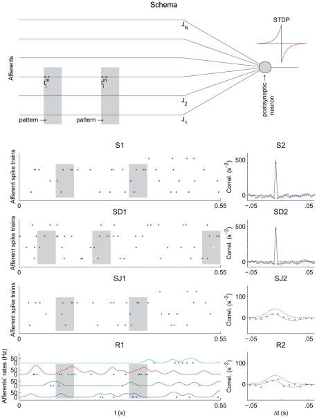
Figure 1. Pattern models and associated cross-correlograms.
Schema: representation of  pattern (bottom) and
  non-pattern (top) inputs that excite, through synapses with weights
  , a postsynaptic neuron equipped with STDP. Grey areas indicate the pattern presentations. For afferent
  ,
,  denotes the latency of the
  spike (Model S) or rate peak (Model R). Below, the left panels (label 1) show the raster plots (each dot indicates a spike) for
  afferents, involving
  pattern inputs. The right panels (label 2) compare predictions (dotted and dashed lines) that correspond to Equation (1) and numerical simulations (circles) for the correlograms. The dashed lines involve an additional approximation compared to the dotted line that is more accurate (compare Equations (S11) in Text S1 and (13), respectively). All patterns have the same latencies
  . (S) Model S with
  , no jitter and
  Hz. Spike times (dots) are the same across presentations for the three pattern inputs (bottom), but not for the fourth non-pattern input (top). The cross-correlogram between second and first afferent exhibits a peak of height
  Hz at
Hz at  ms, cf. Equation (13). (SD) Model S with
  (notice the missing spikes, and the ones added to compensate, in white) and
  Hz, other parameters being the same as in (S). The correlogram is similar to that in (S), in particular its height equal to
  Hz. (SJ) Model SJ with Gaussian jittering at each presentation with spread width
  ms. The correlogram has a peak centered at
  ms and spread width
  , cf. Equation (14). (R) Model R. The rate functions were obtained by convolving the spike trains of (S1) by a Gaussian with amplitude
  and width
  ms (both inside and outside pattern presentations). The rate profiles are thus the same across all pattern presentations for the three pattern inputs (bottom), except for border effects, but not for the non-pattern input (top). From the rate functions, the spikes (dots) are generated using inhomogeneous Poisson processes and thus differ between presentations, both in timing and count. The cross-correlogram between second and first afferents for model R is similar to that in (SJ), cf. Equation (17). The simulated correlograms are averaged over 1000 s for spike patterns (S, SD, SJ) and 50000 s for rate-modulated patterns (R).

