Figure 2.

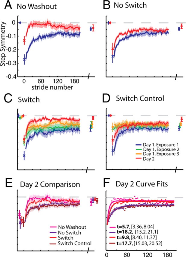
Comparison of step symmetry adaptation across groups. Baseline, first stride, adaptation curves (smoothed by 3 strides) for a portion of training epochs (2–190), and final plateau values are shown. A, No Washout. Mean step symmetry values subtracted from baseline are shown. The first stride is off-set as individual symbols, with mean and SE bars. Average adaptation curves (±SEs in shaded region) for strides 2–190 (∼5 min) of adaptation on day 1 and day 2 are shown in blue and red lines, respectively. Points plotted at the end of these curves represent means (±SE) of the last 30 steps of adaptation on day 1 and 2, also called “plateau” values. B, No Switch. Data are shown as in A, except that this group had a tied-belt period preceding adaptation on day 2 as well (mean of the last 30 s ± SE shown in red at beginning of plot). C, Switch. Data are shown as in B. This group experienced three 5 min exposures to split-belts, interspersed with 5 min washout periods on day 1. Thus, the data plotted in green and yellow represent average values during the second and third exposures to split-belts, respectively. Mean baseline values for exposures 2 and 3 shown at the beginning of this plot represent mean step symmetry in the last 30 s of the washout period preceding that exposure. D, Switch Control. Data are shown as in C. In this group, subjects were given breaks instead of being washed-out between exposures to split-belts, thus baseline data for exposures 2 and 3 are not shown. E, Comparison of day 2 curves. Day 2 adaptation curves and plateau values for each group are shown. Note that all groups reach the same plateau, but differences are seen in the early change of adaptation, with No Washout showing the most improvement, followed by Switch, while No Switch and Switch Control show the least improvement. F, Exponential curve fits for day 2 curves. Average points are shown for the data presented in E. Single exponential time constants (t) with 95% confidence bounds are shown in the legend.