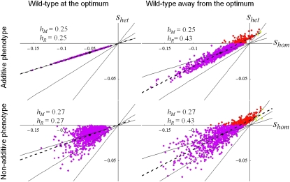
Figure 5.
Heterozygous vs. homozygous fitness effects under different models assumptions. The relationship between homozygous (shom, x-axis) and heterozygous (shet, y-axis) fitness effects of mutations is compared in four situations. Left vs. right: wild type is either at the optimum (so = 0, left) or away from it (so = 0.06, right). Top vs. bottom: mutation effects on the underlying phenotype are either all additive (top, E(ν) = 1/2, συ = 0) or only additive on average, with a random dominance coefficient (bottom, E(ν) = 1/2, συ2 = 0.02, 95% of υ values fall in the range [0.26–0.74]). Dots show the value of (shom, shet) for exact simulations of 1000 mutants, with corresponding values of hM and hR given on each graph. The same color code as in Figure 2 is used: purple, deleterious recessive; yellow, dominant beneficial; red, overdominant. The dashed line is the regression of shet on shom, which is undistinguishable from our prediction (hR and shet0, Equation 13). The black dot gives E(shet) and E(shom). The three plain lines indicate shet = shom/4, shet = shom/2 and shet = shom. hM varies little overall, but hR increases from 1/4 (left) to a value closer to 1/2 (right) when the wild type is far away from the optimum. In the latter situation, overdominant mutations and dominant beneficial mutations are also frequent.

