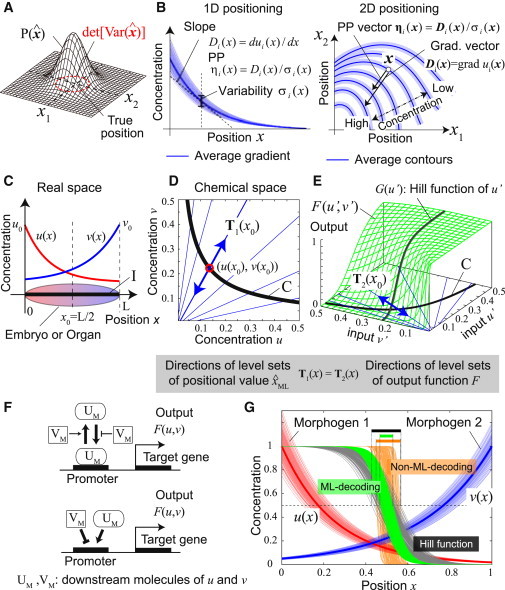
Figure 3.

Definitions of some statistics and biochemical implementation of ML decoding. (A) Precision of positional information is defined as the inverse of the generalized variance of the position estimated ($1/\det \left[\text{Var}\left(\hat{\mathit{x}}\right)\right]$) from the morphogen concentrations that each cell detects. $P\left(\hat{\mathit{x}}\right)$ is the probability distribution of $\hat{\mathit{x}}$. (B) PP vector of morphogen i at position x, η_i (x), is defined as the gradient vector divided by the magnitude of noise, i.e., η_i (x) = (grad u_i(x))/σ_i(x). In one-dimensional positioning (left), it is just a scalar whose sign indicates the direction of the gradient. (C) One-dimensional-positioning by two morphogens with exponential gradients, u(x) = u₀ exp(−αx) and v(x) = v₀ exp(β(x− L)). The values u₀, v₀, and L are the source levels of two morphogens and embryo size. Parameters: (u₀, v₀, L, α, β) = (1,1,1,4,3). (D) Interval I in the real space is mapped into curve C in the chemical space by map (u(x), v(x)). (Blue lines) Directions of the contours of positional values in the chemical space, T₁(x) (see the text for the definition of T₁(x)). (E) A cellular response F(u′,v′). (Blue lines) Directions of dF = 0, T₂(x) = (−∂F/∂v, ∂F/∂u), at each point on curve C. ML decoding can be approximately achieved when T₁(x) ∝ T₂(x). Functions and parameters: F(u′,v′) = u′^h/(u′^h + (Kv′^1/S)^h), G(u′) = u′^h/(u′^h + K₀^h), (h, K, S, K₀) = (4,exp(−0.7/1.1), 1.1, exp (−2)). (F) Biochemical interpretation of Eqs. 8a and 8b. (Top) Promoter regulation of a target gene by a downstream molecule of u (U_M) in which the binding (or unbinding) between U_M and the promoter is repressed (or enhanced) by a downstream molecule of v (V_M). (Bottom) Competitive regulation of a promoter in which U_M and V_M work as an activator and a repressor, respectively. (G) An example of cellular responses. (Thin red and blue curves) Embryo-to-embryo variability of the gradients of two morphogens over 150 embryos. As a noise source, we assumed the variability of morphogen source levels among embryos that obeys two-variable Gaussian distribution with σ₁ = σ₂ = 0.1 and ρ₁₂ = 0.5 (see (4, 19) for the magnitude of noise in real biological systems). (Green and gray curves) Outputs of different embryos when ML-response (F(u′,v′)) and ordinary Hill equation (G(u′)) are adopted, respectively. Parameters for F(u′,v′) and G(u′) are the same as Fig. 3E. Note that the values of both output functions are 0.5 at the center (x = L/2). (Orange curves) An example of the outputs when a non-ML decoding is adopted (where the output function is the same as for the case of green curves but the parameter S(= 0.1) is different from it). ML decoding achieves the minimum variation of the output.