More discussions for granger causality and new causality measures

Abstract

Granger causality (GC) has been widely applied in economics and neuroscience to reveal causality influence of time series. In our previous paper (Hu et al., in IEEE Trans on Neural Netw, 22(6), pp. 829–844, 2011), we proposed new causalities in time and frequency domains and particularly focused on new causality in frequency domain by pointing out the shortcomings/limitations of GC or Granger-alike causality metrics and the advantages of new causality. In this paper we continue our previous discussions and focus on new causality and GC or Granger-alike causality metrics in time domain. Although one strong motivation was introduced in our previous paper (Hu et al., in IEEE Trans on Neural Netw, 22(6), pp. 829–844, 2011) we here present additional motivation for the proposed new causality metric and restate the previous motivation for completeness. We point out one property of conditional GC in time domain and the shortcomings/limitations of conditional GC which cannot reveal the real strength of the directional causality among three time series. We also show the shortcomings/limitations of directed causality (DC) or normalize DC for multivariate time series and demonstrate it cannot reveal real causality at all. By calculating GC and new causality values for an example we demonstrate the influence of one of the time series on the other is linearly increased as the coupling strength is linearly increased. This fact further supports reasonability of new causality metric. We point out that larger instantaneous correlation does not necessarily mean larger true causality (e.g., GC and new causality), or vice versa. Finally we conduct analysis of statistical test for significance and asymptotic distribution property of new causality metric by illustrative examples.

Introduction

Given a set of time series, the topic of how to define causality influence among them has kept philosophers busy for over two thousand years and has yet to be completely resolved. In the literature one of the most popular definitions for causality is Granger causality (GC). Due to its simplicity and easy implementation, GC has been widely used in economics and recently in neuroscience. The basic idea of GC was originally conceived (Wiener 1956) and later formalized by Granger in the form of linear regression model (Granger 1969; Geweke 1982). It can be simply stated as follows: if the variance of the prediction error for the first time series at the present time is not less than the variance of the prediction error by including past measurements from the second time series in the linear regression model, then the second time series can be said to have a causal (driving) influence on the first time series. Reversing the roles of the two time series one repeats the process to address the question of driving in the opposite direction. GC value of is defined to describe the strength of the causality which the second time series has on the first one (Freiwald et al. 1999; Hesse et al. 2003; Ding et al. 2006; Oya et al. 2007; Bressler and Anil 2010). From GC value, it is clear that (i) when there is no causal influence from the second time series to the first one and when there is. This GC definition was extended to frequency domain to show causal influence from one time series on the other one in different frequencies (Geweke 1982; Ding et al. 2006). Several GC or Granger-alike causality metrics in frequency domain have been developed such as spectral GC (Geweke 1982; Ding et al. 2006), PDC (Baccal and Sameshima 2001), RPC (Yamashita et al. 2005), and DTF (Kaminski et al. 2001). To show whether the influence is a direct component or mediated by the third time series, conditional GC is defined (Geweke 1984; Freiwald et al. 1999; Hesse et al. 2003; Ding et al. 2006; Oya et al. 2007; Bressler and Anil 2010). In recent years there has been significant interest to discuss causal interactions between brain areas which are highly complex neural networks in both time and frequency domains (Freiwald et al. 1999; Hesse et al. 2003; Roebroeck et al. 2005; Oya et al. 2007; Wang et al. 2007, 2008; Atmanspacher and Rotter 2008; Gow et al. 2008, 2009; Rajagovindan and Ding 2008; Seth 2008; Cadotte et al. 2009; Zhang et al. 2010).

Although there are wide applications of GC and Granger-alike causality metrics in both time and frequency domains, some shortcomings/limitations of these metrics were pointed out in our recent paper (Hu et al. 2011). To overcome these shortcomings/limitations, we proposed new causality metrics in time and frequency domains. In particular, we emphasized that GC or Granger-alike causality metrics in frequency domain cannot reveal real strength of causality at all and new causality metric in frequency domain has advantages over spectral GC or Granger-alike causality metrics.

In this paper we will focus on time domain and show inherent shortcomings of conditional GC and DC or normalized DC. We will demonstrate that the proposed new causality metric better reveal directed real causality from one time series on the other one than conditional GC and DC or normalized DC. Thus, we must be caution in drawing any conclusion based on GC, conditional GC and DC or normalized DC by noting the shortcomings/limitations of GC (Hu et al. 2011). We will show the influence of one of the time series on the other is linearly increased as the coupling strength is linearly increased by computing GC and new causality values via an example. We will also discuss statistical test for significance and asymptotic distribution property of new causality metric.

Granger causality in time domain

In this section we introduce the well-known Granger causality and conditional Granger causality.

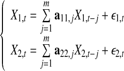
Given two stochastic process X₁(t) and X₂(t) which are assumed to be jointly stationary. Their autoregressive representations are described as

1

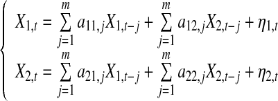
and their joint representations are described as

2

where the noise terms are uncorrelated over time, and η_i have zero means and variances of and The covariance between η₁ and η₂ is defined by

Now consider the first equalities in Eqs. 1 and 2. According to the original formulations (Wiener 1956; Granger 1969), if is less than in some suitable statistical sense, then X₂ is said to have a causal influence on X₁. In this case, the first equality in Eq. 2 is more accurate than that in Eq. 1 to estimate X₁. Otherwise, if then X₂ is said to have no causal influence on X₁. In this case, the two equalities are almost same. Such kind of causal influence called Granger causality (GC) (Ding et al. 2006; Geweke 1982), can be defined by

3

Obviously, when there is no causal influence from X₂ to X₁ and when there is. Similarly, the causal influence from X₁ to X₂ is defined by

4

To show whether the interaction between two time series is direct or is mediated by another recorded time series, conditional Granger causality (Ding et al. 2006; Geweke 1984), was defined by

5

where and are variances of two noise terms, and η₃, of the following two joint autoregressive representations:

6

and X_1,t = 

7

According to this definition, means that no further improvement in the prediction of X₁ can be expected by including past measurements of X₂. On the other hand, when there is still a direct component from X₂ to X₁, the past measurements of X₁, X₂, X₃ together result in better prediction of X₁, leading to and

For conditional GC, we point out one important property as follows.

Property 1 Consider the following model

8

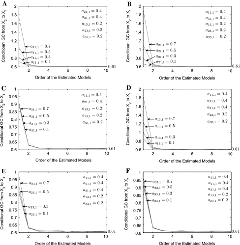
where 0 < a_i1,1, a_i3,1 < 0.7, i = 1, 2, 3 and for simplicity η₁, η₂, η₃ are assumed to be independent white noise processes with zero mean and variances Figure 1 shows for Model (8) under different parameters a_i1,1 and a_i3,1. When we calculate conditional GC it should be pointed out that for each specific Model (8) we generate a data set of 200 realizations of 10,000 time points. For each realization, we estimate AR models (joint representations Model (6) and Model (7)) with the order of 8 by using the least-squares method and calculate conditional GC where the order 8 fits well for all examples throughout the paper (see Fig. 1a and b from which one can see keeps steady when the order of the estimated models is >8). Then we obtain the average value across all realizations and get From Fig. 1 one can clearly see that has nothing to do with parameters a_i1,1 and a_i3,1, i = 1, 2, 3 (of course, choices of parameters a_i1,1 and a_i3,1 are such that Model (8) does not diverge).

Fig. 1.

a as a function of the order of the estimated models for Model (8) when a_21,1 = a_31,1 = 0.4, a_13,1 = a_23,1 = a_33,1 = 0.2 and a_11,1 changes from 0.1 to 0.7. b as a function of the order of the estimated models for Model (8) when a_11,1 = a_31,1 = 0.4, a_13,1 = a_23,1 = a_33,1 = 0.2 and a_21,1 changes from 0.1 to 0.7. c as a function of the order of the estimated models for Model (8) when a_11,1 = a_21,1 = 0.4, a_13,1 = a_23,1 = a_33,1 = 0.2 and a_31,1 changes from 0.1 to 0.7. d as a function of the order of the estimated models for Model (8) when a_11,1 = a_21,1 = a_31,1 = 0.4, a_23,1 = a_33,1 = 0.2 and a_13,1 changes from 0.1 to 0.7. e as a function of the order of the estimated models for Model (8) when a_11,1 = a_21,1 = a_31,1 = 0.4, a_13,1 = a_33,1 = 0.2 and a_23,1 changes from 0.1 to 0.7. f as a function of the order of the estimated models for Model (8) when a_11,1 = a_21,1 = a_31,1 = 0.4, a_13,1 = a_23,1 = 0.2 and a_33,1 changes from 0.1 to 0.7. From a–f one can see that a) keeps steady and converges to 0.61 when the order p > 4. b has nothing to do with parameters a_i1,1 and a_i3,1

By the conditional GC definition (5), we know that conditional GC explicitly measures the degree to which X₂ predicts X₁ over and above the degree to which X₁ already predicts itself and X₃ predicts X₁, the influence of X₁ on itself (i.e. the coefficients a_i1,1) and X₃ on X₁ (i.e. the coefficients a_i3,1) are factored out and quite correctly makes no difference to the result. So, according to the conditional GC definition (5) the above property is true.

In general GC is useful to show whether or not theoretically there is directional interaction between two neurons or among three neurons. When there exists causal influence, a question is arising: does GC value reveals the real strength of causality? to answer this question, let’s consider the following simple model

9

where η₁ and η₂ are two independent white noise processes with zero mean and a_12,1a_21,1 ≠ 0. From Model (9) one can get

10

So, GC value

11

or equivalently,

12

which is only related to the last two noise terms and has nothing to do with the first term. It is noted that all of three terms make contributions to current X_1,t, and a_12,1a_21,1X_1,t−2 must have causal influence on X_1,t and must be considered to illustrate real causality. Especially, when we have X_1,t = a_12,1a_21,1X_1,t−2 + η_1,t and Since a_21,1X_1,t−2 comes from X_2,t−1 we can surely know that X₂ has real nonzero causality on X₁ due to a_12,1a_21,1 ≠ 0. Thus, GC value may not reveal real causality at all. As such, the definition has its inherent shortcomings and/or limitations to illustrate the real strength of causality. Please refer to Remark 1 (Hu et al. 2011) for the detailed discussions.

New causality

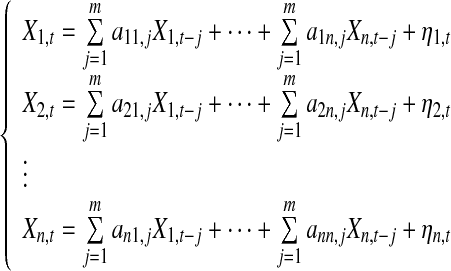
Due to the shortcomings and/or limitations of GC, we next give a new definition for causality anaylsis of multivariate time series. Let’s consider the following general model:

13

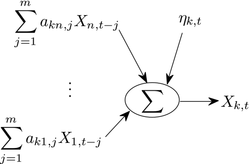
where are n time series, has zero mean and variance of and Based on Eq. 13, Fig. 2 clearly shows contributions to X_k,t, which includes and the noise term η_k,t where the influence from is causality from X_k’s own past values. Each contribution plays an important role in determining X_k,t. If occupies larger portion among all those contributions, then X_i has stronger causality on X_k, or vice versa. Thus, a good definition for causality from X_i to X_k in time domain should be able to describe what proportion X_i occupies among all these contributions. This is a general guideline for proposing any causality method (i.e., all contributions must be considered). For Eq. 10, let’s define

14

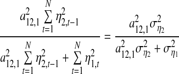
which is summation of two noise terms and each noise term makes contributions to To describe what proportion η₂ occupies in we define

15

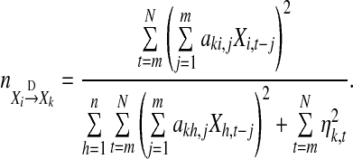
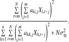
which is the same as GC defined in Eq. 12. Therefore, here in nature GC is actually defined based on the noise model (14) and follows the above guideline. Motivated by this idea, we can naturally extend the noise model (14) to the kth equation of Model (13) and define a new direct causality from X_i to X_k as follows:

16

When N is large enough,

Then, Eq. 16 can be approximated as

17

Throughout the paper, we always assume that N is large enough so that is always defined as Eq. 17.

Fig. 2.

Contributions to X_k,t

New causality based on Eq. 10 can be written as

18

which describes what proportion X₂ occupies among two contributions in X₁ (see Eq. 10). Note that for (10) GC is proposed based on Model (14) and describes what proportion η₂ occupies among two contributions in (see Eq. 15). Thus GC actually reveals causal influence from η₂ to it does not reveal causal influence from X₂ to X₁ at all by noting that is only partial information of X₁, i.e., the noise terms a_12,1η_2,t−1 + η_1,t. One can see that new causality definition based on Eq. 10 is a natural extension of GC definition based on Eq. 14 as far as the concept of proportion is concerned (in this way, our new causality definition has a rather sound conceptual or theoretical basis). But, as said above, the equivalent GC describes what the proportion η₂ occupies in of Eq. 14 and new causality describes what the proportion X₂ occupies in X₁ of Eq. 10. Thus, they are two totally different concepts, that is, the equivalent GC reveals causal influence from η₂ to but new causality indeed reveals causal influence from X₂ to X₁. Obviously, one cannot use causal influence value from η₂ to (involving partial information of X₁, i.e., the noise terms a_12,1η_2,t−1 + η_1,t) to express causality influence value from X₂ to X₁ (involving complete information, i.e.,the noise terms a_12,1η_2,t−1 + η_1,t plus a_12,1a_21,1X_1,t−2). Any causality definition (like traditional GC) only using partial information of X₁ inevitably leads to misinterpretation result. In addition to some important points shown in Remark 2 (Hu et al. 2011), next we give some more comments for new causality in the following remark.

Remark 1 (1) Let the transfer function of Model (13) be H(f) = [H_ij(f)]_n × n. RPC (Yamashita et al. 2005) is used to reveal causality influence from X_j to X_i at frequency f and is defined as

19

where the power spectrum

20

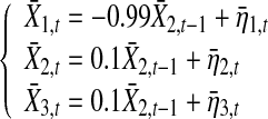
Equation 20 indicates that the power spectrum of X_i,t at frequency f can be decomposed as to n terms each of which can be interpreted as the power contribution of the jth innovation η_j,t transferring to X_i,t via the transfer function H_ij(f). RPC can be regarded as a ratio of the power contribution of the innovation η_j,t on the power spectrum of X_i,t to the power spectrum From this point of view, this ratio also provides a strong motivation (or theoretical basis) to define the proposed new causality metric Eq. 16 for multivariate time series. However, as pointed out in Remark 6 (Hu et al. 2011) RPC has inherent shortcomings/limitations and cannot reveal real causality influence at all.(2) Consider the following two models

21

and

22

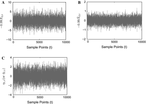
where η₁, η₂ and η₃ are three independent white noise processes with zero mean and variances and the initial conditions and From both of Models (21) and (22) it can be seen that there are no direct causality from X₃ to X₁, so, Moreover, based on Property 1, are same for both of Models (21) and (22). We can obtain for both of Models (21) and (22), for Model (21), and for Model (22). Figure 3 shows trajectories and η₁ for one realization of Model (21) and Model (22). From Fig. 3a and c one can clearly see that amplitudes of −0.99X₂ are much larger than that of η₁ and the contribution from −0.99X_2,t−1 occupies much larger portion compared to that from η_1,t, as a result, the causal influence from X₂ to X₁ occupies a major portion compared to the influence from η₁ and the real strength of causality from X₂ to X₁ should have higher value. This fact is real. Our causality value for Model (21) is consistent with this fact. Similarly, from Fig. 3b and c one can clearly see that amplitude of is much smaller than that of η₁ and the contribution from occupies much smaller portion compared to that from η_1,t, as a result, the causal influence from to occupies a rather small portion compared to the influence from η₁ and the real strength of causality from to should have smaller value. This fact is also real. 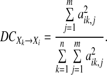Our causality value for Model (22) is consistent with this fact. However, conditional GC always equals to 0.092 for both of Models (21) and Eq. 22 and does not reflect such kind of changes at all, and violates above two real facts. These results show that the conditional GC definition (5) does not reveal real strength of direct causality from X₂ to X₁ at all for Models (21) and (22), our new causality definition very reasonably reflects the real strength of the direct causality.(3) An alternate time-domain metric namely direct causality (DC) has been proposed earlier (Kaminski et al. 2001) which quantifies causality based on the AR coefficients

or the following normalized measure

23

Since the AR coefficients themselves represent the coupling strength, now a question is arising: would this normalized measure suffice to reveal the real causality of two time series? Unfortunately, the answer is no. Let’s take a look at the following model:

24

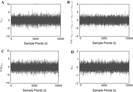
where η₁, η₂ and η₃ are three independent white noise processes with zero mean and variances For Models (24) we can obtain and Figure 4 shows trajectories of X_1,t, 0.9(− X_2,t−1 + X_2,t−2 − X_2,t−3 + X_2,t−4), 0.9X_3,t, and η_1,t for one realization of Model (24). From Fig. 4a–d one can clearly see that amplitudes of 0.9X₃ are much larger than that of η_1,t and 0.9(− X_2,t−1 + X_2,t−2 − X_2,t−3 + X_2,t−4), and the contribution from 0.9X₃ occupies much larger portion compared to that from η_1,t and 0.9(− X_2,t−1 + X_2,t−2 − X_2,t−3 + X_2,t−4). As a result, the causal influence from X₂ to X₁ occupies a small portion compared to the influence from 0.9X₃ and the real strength of causality from X₂ to X₁ should have smaller value. This fact is real. Our causality value for Model (24) is consistent with this fact. 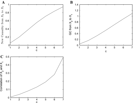However, for Model (24) violates the real fact. These results show that the direct causality definition (23) does not reveal real strength of direct causality from X₂ to X₁ at all for Model (24), our new causality definition reflects the real strength of the direct causality very reasonably.(4) It should be noted that the influence of one of the time series on the other is linearly increased as the coupling strength is linearly increased. Let’s consider the following bivariate AR process with 5 levels of coupling strength:

25

where η₁ and η₂ are two independent white noise processes with zero mean and variances From Eq. 25 one can see that the coupling strength of X₂ on X₁ is linearly increased as the parameter c increases. The true causality of X₂ on X₁ should increase as the parameter c increases. The estimated causality measures (new causality and GC) against the parameter c are shown in Fig. 5a and b, respectively, from which one can clearly see that both of two metrics indicate the increasing true causality as the true coupling strength (i.e., the parameter c) increases.(5) Figure 5c shows the increasing instantaneous correlation (i.e., zero-lag influence) of two time series as the parameter c increases. Combining Fig. 5a and b with c we can conclude that the increasing instantaneous correlation leads to the reasonable increasing new causality and GC. However, in general this conclusion may not be true. It is well known that in general there may be no relationship between true causality and correlation. In other words, larger correlation does not necessarily mean larger true causality, or vice versa. Therefore, it is meaningless to discuss whether new causality or GC will be affected by correlation.

Fig. 3.

For one realization of Model (21) and Model (22) where and trajectories for and η_1,t are plotted: a −0.99X_2,t’s trajectory for Model (21). b’s trajectory for Model (22). c η_1,t’s or ’s trajectory

Fig. 4.

For one realization of Model (24), trajectories for X_1,t, 0.9(− X_2,t−1 + X_2,t−2 − X_2,t−3 + X_2,t−4), 0.9X_3,t, and η_1,t are plotted: a Trajectory for X_1,t. b Trajectory for 0.9(− X_2,t−1 + X_2,t−2 − X_2,t−3 + X_2,t−4). c Trajectory for 0.9X_3,t. d Trajectory for η_1,t

Fig. 5.

Causality (or correlation) vs the parameter c for Model (25). a New causality of X₂ on X₁ vs the coupling strength (i.e., the parameter c). b GC of X₂ on X₁ vs the coupling strength (i.e., the parameter c). c Correlation of X₂ and X₁ vs. the coupling strength (i.e., the parameter c)

Statistical test for significance

Since new causality metric has a highly nonlinear relation to the time series data, it makes tests of significance difficult to perform. In this section, we use the same technology (Kaminski et al. 2001) to deal with this problem; that is, we first create a surrogate data set (Theiler et al. 1992) for each channel, we then fit a model to this surrogate data set and calculate new causality metric. Repeating this process many time, we can obtain an empirical distribution for the metric. Based on this distribution we can then evaluate the significance of the causal metric derived from the actual data. We use the following model to illustrate the process.

26

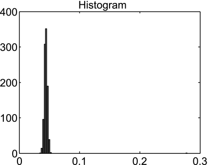
where η₁ and η₂ are two independent white noise processes with standard normal distribution. For a simulated data of a realization of Model (26), we produce surrogate data (i.e., perform random and independent shuffling of X₁ and X₂). We then estimate a joint regression model (2) with m = 6 to fit the shuffled data and calculate new causality value. Carrying out the procedure for 1,000 such independently shuffled data sets we can construct an empirical distribution for the new causality values. Since the shuffling procedure destroys all the temporal structure in the data, this empirical distribution gives the variability for the new causality values when the null hypothesis of no causal influence is true.

Figure 6 shows Histogram of new causality values based on the original simulated data and 1000 surrogate data. One can see that the new causality value (=0.275) based on the original simulated data is statistically significant (P < 0.001).

Fig. 6.

Histogram of new causality values resulting from 1,000 surrogate data sets

Asymptotic distribution property

It is well known that the asymptotic distribution of GC metric under the null hypothesis of zero causality is known (it is a χ ²-distribution) (Geweke 1982). Now a question is arising: what is asymptotic distribution for new causality metric under the null hypothesis of zero causality? For new causality metric can we derive the similar asymptotic distribution property as GC metric? In general it is difficult to discuss this issue because of complexity of new causality definition. But in the following example we find that new causality metric has χ²(1)-distribution as GC metric.

27

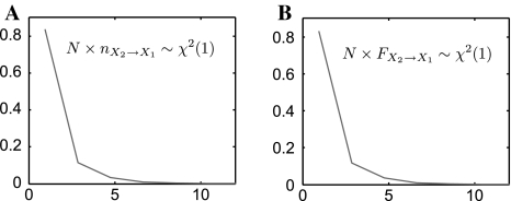
where η₁ and η₂ are two independent white noise processes with standard normal distribution, (i.e., N = 10,000). For each realization of Model (27) we set m = 1 to estimate the autoregression Model (1) and the joint regression Model (2), then based on the two estimated models we calculate new causalty and GC This process is repeated by N = 10,000 times. Finally we plot large-sample distributions for and in Fig. 7a and b, respectively. One can see probability density functions for both new causality and GC follow χ²(1)-distribution. In general, as for whether or not follows a χ²-distribution under the null hypothesis of zero causality keeps unknown and is left for further study in near future.

Fig. 7.

Probability distribution functions (PDF). a PDF for new causality metric. b PDF for GC metric

Conclusions

In this paper, we further make more discussions for GC or Granger-alike causality and new causality metrics by following our previous paper (Hu et al. 2011) and focus on time domain. In addition to the previous motivation for introducing new causality metric in time domain, we provide additional strong motivation (or theoretical basis) to the proposed metric for multivariate time series. After introducing one property for conditional GC, we point out the inherent shortcomings/limitations of conditional GC and demonstrate that it cannot reveal directed causal influence from one time series to the other one among three time series. We also point out the shortcomings/limitations of Granger-alike causality, i.e., DC or normalized DC metric and show that it cannot disclose directed causality influence at all for multivariate time series. Furthermore, all these shortcomings/limitations demonstrate reasonability and advantages of new causality metric. Therefore, researchers must be caution in drawing any conclusion based on DC (or normalized DC) value and conditional GC value. By calculating GC and new causality values for an example we show the influence of one of the time series on the other is linearly increased as the coupling strength is linearly increased. Finally for new causality metric in time domain we analyze statistical test for significance and show significance level for a simulated data, meanwhile we conduct analysis for asymptotic distribution property by an examples in which both GC and new causality metrics follow χ²(1)-distribution. However, in general, as for whether or not new causality metric follows a χ²-distribution under the null hypothesis of zero causality keeps unknown and is left for further study in near future. Thus our proposed new causality metrics in time and frequency domains may have wide applications in economics and neuroscience.

References

- Atmanspacher H, Rotter S. Interpreting neurodynamics: concepts and facts. Cogn Neurodyn. 2008;2:297–318. doi: 10.1007/s11571-008-9067-8. [DOI] [PMC free article] [PubMed] [Google Scholar]
- Baccal LA, Sameshima K. Partial directed coherence: a new concept in neural structure determination. Biol Cybern. 2001;84(6):463–474. doi: 10.1007/PL00007990. [DOI] [PubMed] [Google Scholar]
- Bressler SL, Anil KS (2010) Wiener-Granger causality: a well established methodology. NeuroImage (in press) [DOI] [PubMed]
- Cadotte AJ, Mareci TH, DeMarse TB, et al. Temporal lobe epilepsy: anatomical and effective connectivity. IEEE Trans Neural Syst Rehabil Eng. 2009;17(3):214–223. doi: 10.1109/TNSRE.2008.2006220. [DOI] [PubMed] [Google Scholar]
- Ding M, Chen Y, Bressler SL. Granger causality: basic theory and applications to neuroscience. In: Schelter B, Winterhalder M, Timmer J, editors. Handbook of time series analysis. Weinheim: Wiley; 2006. pp. 437–460. [Google Scholar]
- Freiwald WA, Valdes P, Bosch J, et al. Testing non-linearity and directedness of interactions between neural groups in the macaque inferotemporal cortex. J Neurosci Methods. 1999;94(1):105–119. doi: 10.1016/S0165-0270(99)00129-6. [DOI] [PubMed] [Google Scholar]
- Geweke J. Measurement of linear-dependence and feedback between multiple time series. J Am Stat Assoc. 1982;77(378):304–313. doi: 10.2307/2287238. [DOI] [Google Scholar]
- Geweke J. Measures of conditional linear dependence and feedback between time series. J Am Stat Assoc. 1984;79(388):907–915. doi: 10.2307/2288723. [DOI] [Google Scholar]
- Granger CWJ. Investigating causal relations by econometric models and cross-spectral methods. Econometrica. 1969;37(4):424–438. doi: 10.2307/1912791. [DOI] [Google Scholar]
- Gow DW, Segawa JA, Alfhors S, et al. Lexical influences on speech perception: a Granger causality analysis of MEG and EEG source estimates. Neuroimage. 2008;43(3):614–623. doi: 10.1016/j.neuroimage.2008.07.027. [DOI] [PMC free article] [PubMed] [Google Scholar]
- Gow DW, Keller CJ, Eskandar E, et al. Parallel versus serial processing dependencies in the perisylvian speech network: a Granger analysis of intracranial EEG data. Brain Lang. 2009;110(1):43–48. doi: 10.1016/j.bandl.2009.02.004. [DOI] [PMC free article] [PubMed] [Google Scholar]
- Hesse W, Oller M, Arnold M, et al. The use of time-variant EEG Granger causality for inspecting directed interdependencies of neural assemblies. J Neurosci Methods. 2003;124(1):27–44. doi: 10.1016/S0165-0270(02)00366-7. [DOI] [PubMed] [Google Scholar]
- Hu S, Dai G, Worrell GA, et al. Causality analysis of neural connectivity: critical examination of existing methods and advances of new methods. IEEE Trans on Neural Netw. 2011;22(6):829–844. doi: 10.1109/TNN.2011.2123917. [DOI] [PMC free article] [PubMed] [Google Scholar]
- Kaminski M, Ding M, Truccolo-Filho W, et al. Evaluating causal relations in neural systems: Granger causality, directed transfer function and statistical assessment of significance. Biol Cybern. 2001;85:145–157. doi: 10.1007/s004220000235. [DOI] [PubMed] [Google Scholar]
- Oya H, Poon PWF, Brugge JF, et al. Functional connections between auditory cortical fields in humans revealed by Granger causality analysis of intra-cranial evoked potentials to sounds: comparison of two methods. Biosystems. 2007;89:198–207. doi: 10.1016/j.biosystems.2006.05.018. [DOI] [PubMed] [Google Scholar]
- Rajagovindan R, Ding M. Decomposing neural synchrony: toward an explanation for near-zero phase-lag in cortical oscillatory networks. Plos one. 2008;3(11):e3649. doi: 10.1371/journal.pone.0003649. [DOI] [PMC free article] [PubMed] [Google Scholar]
- Roebroeck A, Formisano E, Goebel R. Mapping directed influence over the brain using Granger causality and fMRI. Neuroimage. 2005;25(1):230–242. doi: 10.1016/j.neuroimage.2004.11.017. [DOI] [PubMed] [Google Scholar]
- Seth AK. Causal networks in simulated neural systems. Cogn Neurodyn. 2008;2:49–64. doi: 10.1007/s11571-007-9031-z. [DOI] [PMC free article] [PubMed] [Google Scholar]
- Wiener N. The theory of prediction. In: Beckenbach EF, editor. Modern mathematics for engineers, Chap. 8. New York: McGraw-Hill; 1956. [Google Scholar]
- Wang X, Chen Y, Ding M. Estimating Granger causality after stimulus onset: a cautionary note. Neuroimage. 2008;41(3):767–776. doi: 10.1016/j.neuroimage.2008.03.025. [DOI] [PMC free article] [PubMed] [Google Scholar]
- Wang X, Chen Y, Bressler SL, et al. Granger causality between multiple interdependent neurobiological time series: blockwise versus pairwise methods. Int J Neural Syst. 2007;17(2):71–78. doi: 10.1142/S0129065707000944. [DOI] [PubMed] [Google Scholar]
- Zhang L, Zhong G, Wu Y, et al. Using granger-geweke causality model to evaluate the effective connectivity of primary motor cortex, supplementary motor area and cerebellum. J Biomed Sci Eng. 2010;3:848–860. doi: 10.4236/jbise.2010.39115. [DOI] [PMC free article] [PubMed] [Google Scholar]
- Yamashita O, Sadato N, Okada T, et al. Evaluating frequency-wise directed connectivity of BOLD signals applying relative power contribution with the linear multivariate time-series models. Neuroimage. 2005;25(2):478–490. doi: 10.1016/j.neuroimage.2004.11.042. [DOI] [PubMed] [Google Scholar]