Segmentation of 3D Radio Frequency Echocardiography Using a Spatio-temporal Predictor

Abstract

This paper presents an algorithm for segmenting left ventricular endocardial boundaries from RF ultrasound. Our method incorporates a computationally efficient linear predictor that exploits short-term spatio-temporal coherence in the RF data. Segmentation is achieved jointly using an independent identically distributed (i.i.d.) spatial model for RF intensity and a multiframe conditional model that relates neighboring frames in the image sequence. Segmentation using the RF data overcomes challenges due to image inhomogeneities often amplified in B-mode segmentation and provides geometric constraints for RF phase-based speckle tracking. The incorporation of multiple frames in the conditional model significantly increases the robustness and accuracy of the algorithm. Results are generated using between 2 and 5 frames of RF data for each segmentation and are validated by comparison with manual tracings and automated B-mode boundary detection using standard (Chan and Vese-based) level sets on echocardiographic images from 27 3D sequences acquired from 6 canine studies.

1. Introduction

Quantitative analysis of regional left ventricular deformation from echocardiography can detect ischemia and ischemic injury and offers important prognostic information. One important area of quantitative analysis is speckle tracking in high frame-rate radio-frequency (RF) echocardiography. Speckle tracking yields dense estimates of displacement, strain, and strain rate (Lubinski et al., 1999). Speckle tracking methods assume that the acoustic medium in the neighborhood of a point is homogeneous, but this assumption fails at blood-tissue boundaries. Furthermore, speckle tracking methods are computationally intensive. RF segmentation prior to speckle tracking can substantially alleviate both problems: it can indicate where the blood-tissue boundary is located, thus alerting the speckle tracking of possible failure. The segmentation can also provide a geometric constraint to reduce the amount of data to be processed since speckle need not be tracked in the blood pool. The goal of this paper is to report a robust segmentation strategy for RF echocardiography data that can be used as a preprocessing step in RF phase-based speckle tracking.

In ultrasound, segmentation of the endocardium is particularly challenging due to characteristic artifacts such as attenuation, shadows, and dropout and is further complicated by spatially varying contrast (Noble and Boukerroui, 2006). Signal dropout is particularly challenging as it leads to gaps in boundaries that must be bridged by segmentation algorithms (Qian and Tagare, 2006). Using high frame rate (> 30 fps) RF ultrasound can help overcome problems with spatio-temporal contrast variation and dropout because the RF signal exhibits long term temporal coherence in the myocardium and this coherence is robust to contrast variation. This coherence is exploited by state-of-the-art RF speckle tracking through the analysis of complex correlations and is documented in the ultrasound physics literature (Lubinski et al., 1999).

In a research setting, the RF data is digitally stored and output before the image is envelope detected, log-compressed, and scan-line converted to form a B-mode image. Thus, there is a close relation between RF and B-mode segmentations. There is increasing access to the raw RF signal motivated by its intended wide use in the elastography community. As previously mentioned, there is also a great deal of clinical and scientific interest in speckle tracking in 3D echocardiography. The increasing role of RF in ultrasound imaging research is supported by industry advances as well. ¹ Finally, RF data will become more available as 3D high-resolution speckle tracking becomes more interesting clinically.

1.1. Literature Review

There are very few reports of RF data segmentation in the literature. Yan et al. (2007) and Nillesen et al. (2009) present the maximum correlation coefficient (MCC) image, a derived parameter in speckle tracking, as a useful feature for segmentation. These methods suffer from the fact that computation of the MCC images is extremely computationally burdensome. Dydenko et al. (2003) introduce a spectral autoregressive model and a velocity based model for RF segmentation. The authors show that the variance of the velocity field is a meaningful parameter for segmentation. This method is also computationally expensive, especially in the calculation of velocity estimates.

The key observation in all of the above research is that the temporal coherence in the blood pool and myocardium have different patterns and that this difference can be used for segmentation. We too exploit this principle, although we use linear prediction, which is computationally simpler than calculating the MCC image or velocity estimates. Experiments show that this simple model provides accurate segmentations. That is the main contribution of this paper.

Before proceeding with details, we would like to emphasize the difference between the use of temporal image coherence as a segmentation feature and the use of temporal image information to track segmentation. Although both use multiple frames of the image sequence, the former uses temporal information to segment a single frame while the latter uses temporal information to propagate the segmentation from frame to frame. The two are quite distinct and should not be confused. There have been several extensions of level set segmentation methods for propagating the segmentation, including extensions of Chan and Vese (2001), to incorporate motion. These are comprehensively reviewed in Cremers et al. (2007). Recent advances also include Fundana et al. (2008) and Paragios and Deriche (2005).

In Pearlman et al. (2010) we introduce Segmentation Using a Linear Predictor (SLiP) where spatio-temporal information is exploited by using the residues of a linear predictor as a basis for segmentation. In Pearlman et al. (2011) we introduce the use of a conditional probability model for two image frames that yields an independent identically distributed (i.i.d) spatial term for the frame being segmented and a two-frame linear prediction based term (cSLiP). We generalize our previous work by introducing a model that incorporates an arbitrary number of frames. We refer to this algorithm as multiframe SLiP (mSLiP). The image is modeled with a conditional probability relating the frame we wish to segment to an ensemble of future time points.

1.2. Overview of Proposed Method

A schematic overview of our segmentation approach is provided in Fig. 1. The two features that are chosen for our segmenter are absolute speckle intensity (single-frame phase contributes no spatial information) and spatio-temporal coherence from complex RF data. Information from both segmentation features are used jointly to segment the endocardium.

Figure 1.

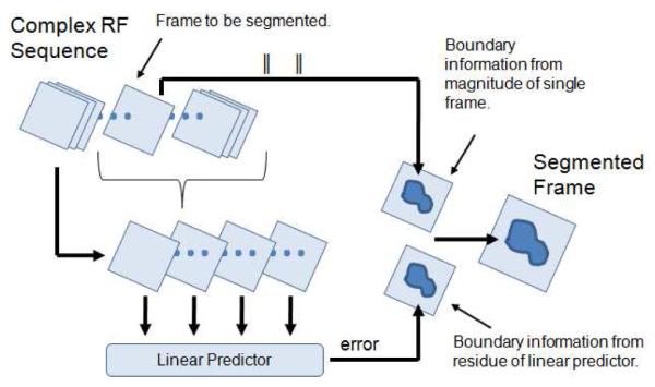
Overview of segmentation method.

In our approach, subsequent frames are related to each other with a linear predictor. The predictor coarsely models the motion of the myocardium and blood pool and its residues, which are used as a segmentation feature, are directly related to the variance of the velocity adopted in Dydenko et al. (2003). Also, the spatio-temporal predictor is a more robust segmentation feature than the single-frame autoregressive model in Dydenko et al. (2003). While the autoregressive fit will vary significantly across the image, the temporal coherence in the signal leads to a more consistent fit that can be used to segment the whole boundary. Finally, the coefficients of the predictor are represented as a tensor product to simplify computations.

The primary contribution of our new multiframe predictor based algorithm is that it extends the theory behind our previous model such that our segmentation feature makes use of significantly more data, greatly improving the segmentation accuracy. We adopt a maximum a posteriori (MAP) approach with a level set active contour. We compare our method to a traditional Chan-Vese intensity based level set segmenter on B-mode images (Chan and Vese, 2001). We also analyze the benefit of using between two and five frames in the mSLiP segmentation to determine how many frames contribute to more accurate segmentations of our data set. Quantitative validation is performed by comparing our results with manual segmentations. Additional validation is performed by analyzing the algorithm’s sensitivity to the weights on priors in the model.

2. Materials and Methods

2.1. Signal Model

Origins of temporal coherence in RF data

The interaction of the base-band RF signal with the blood pool and the myocardium is of interest for this work. The blood pool is made up of plasma and other elements that are much smaller than the wavelength of the ultrasound, while the myocardium is primarily made up of muscular fibers interspersed with blood vessels. The fibers make up 90% of the myocardial tissue and are thus responsible for most of the received signal (Shung and Thieme, 1993). The regular structure of the fibers is responsible for the temporal coherence in the data that we exploit with our algorithm. Likewise, the lack of regular structure in the blood pool causes the signal to rapidly decorrelate. When data is acquired at a high frame rate, the motion of the speckle between frames is of the same order of magnitude as the motion of the boundaries. As a result, a single linear predictor for each medium (blood pool and myocardium) can capture spatio-temporal coherence in the RF data.

Preprocessing

The input pulse produced by the ultrasound machine is a real, bandlimited signal. Because the effects of transmission and reflection in ultrasound are linear, the received signal is also real and bandlimited and can be recovered by coherent demodulation (Langton, 1999). Demodulation gives a vector image consisting of an in-phase and a quadrature component, and is referred to as the analytic signal. It is this vector image that we are interested in segmenting.

Data Visualization

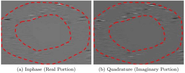
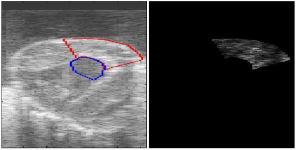
An example slice of a complex analytic image containing myocardium and blood pool is shown in Figure 2. In contrast to B-mode images, the analytic image is not log-compressed. For this reason, the boundaries in Figure 2 are difficult to observe. A manual segmentation is overlaid in red to delineate the myocardium and blood pool. To avoid figures with poor contrast, such as in Figure 2, the results of our work, reported in Section 3, will be overlaid on the B-mode data where the contrast between the myocardium and blood pool is more obvious.

Figure 2.

Slice of 3D analytic image containing myocardium and blood pool (vertical is axial direction and horizontal is angular). Manual segmentation overlaid to aid in visual inspection. Note that the analytic image has not been log-compressed to reduce the dynamic range for visualization purposes (unlike B-mode data).

2.2. Temporal Coherence as a Segmentation Feature

There are two “features” in the data that help us segment the endocardium. The first is the difference between the spatio-temporal coherence in the RF signal of the myocardium and the blood pool. The second is the difference in the absolute backscatter from the myocardium and the blood. Absolute backscatter is readily apparent in the B-mode signal. We use both these features – temporal coherence in the RF signal is exploited by a linear model that operates across multiple frames, while the absolute backscatter is exploited by using the B-mode in the frame to be segmented.

It takes some work to use the RF and the B-mode consistently in a probabilistic framework while keeping the method computationally tractable. Our goal is to augment single-frame B-mode segmentation to incorporate temporal phase-coherence in the RF, so we seek to model each segmentation feature separately. Suppose I¹ is the complex valued 3D frame to be segmented and {I², …, I^L} are subsequent frames. We are thus interested in modeling the probability distribution, p (I¹ | I², …, I^L, Ψ), where Ψ is a vector containing the segmentation and auxiliary parameters. It is difficult to tease out a model for only the gray levels of I¹ from this model, so our approach is the following:

$$p(I^1\mid I^2,\dots ,I^L,\Psi )\propto p(I^L,\dots ,I^2\mid I^1,\Psi )\cdot \Pi (I^1\mid \Psi ),$$ (1)

where Π is a marginal distribution for I¹. Using Bayes Rule the right hand side of equation (1) is a conditional forward model and a marginal. In the following sections, the conditional will be used to relate RF frames by means of a linear Markov model. The marginal will be used to model the gray levels of the envelope in Section 2.6. The conditional is used to exploit spatio-temporal coherence in the RF while the marginal is used to exploit absolute backscatter from the B-mode.

Segmentation is accomplished by minimizing the following energy:

$$\begin{array}{cc}\hfill \underset{\Psi }{\arg \min }E(I_k^1,\dots ,I_k^L,\Psi )& =\underset{\Psi }{\arg \min }-\log p(I_k^1,\dots ,I_k^L,\Psi )\hfill \\ \hfill & +{\lambda }_{AL}{E}_{AL}\left(\Psi \right)+{\lambda }_S{E}_S\left(\Psi \right)\hfill \end{array}$$ (2)

where λ_ALE_AL(Ψ) and λ_SE_S(Ψ) are priors that are explained in detail in Section 2.9. The segmentation probability is developed in the following sections.

2.3. Linear Predictor

We now define the forward linear model we use to relate frames in the RF image sequence. The domain of I¹ is Ω and C is a boundary between two disjoint regions in the image, Ω₁ and Ω₂, where Ω = Ω₁ ⋃ Ω₂. The voxels of {I¹, …, I^L} are indexed by k, where k runs over the voxels of each image in {I¹, …, I^L} in a scan line fashion. Therefore, the k^th voxel in image I^r is given by $I_k^r$. We represent C with an implicit level set function, ϕ, where C = {k | ϕ (k) = 0} The forward linear model we introduce in the following captures the effects of spatio-temporal coherence in the data.

We model the complex valued $I_k^r$ linearly using a neighborhood of voxels around $I_k^{r+1}$ with complex coefficients and a residue. A diagram of the predictor is shown in Figure 3. The voxels in a neighborhood around $I_k^r$ are used to predict $I_k^{r+1}$and, similarly, the voxels in a neighborhood around $I_k^{r+1}$ are used to predict $I_k^{r+2}$.

Figure 3.

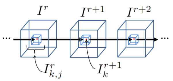
Linear predictor for point k.

We assume that the process, {I¹, …, I^L}, can be treated as locally stationary in time because the sequence is acquired at a high frame rate (> 30 fps) relative to the motion of the structures being imaged. Thus, the same prediction coefficients are used for all predictors. Also, the coefficients do not vary spatially, but rather are fixed within the blood pool and myocardium. This is sufficient for segmentation because the blood pool decorrelates quickly. The residues of the linear predictors are given by

$$e_k^r=\{\begin{array}{cc}{I}_k^{r+1}-\sum _{j\in Nbd\left(k\right)}{\alpha }_{1,j}\mathcal{R}e\left\{I_j^r\right\}-i\sum _{j\in Nbd\left(k\right)}{\beta }_{1,j}\mathcal{I}m\left\{I_j^r\right\},\hfill & k\in {\Omega }_1,\hfill \\ I_k^{r+1}-\sum _{j\in Nbd\left(k\right)}{\alpha }_{2,j}\mathcal{R}e\left\{I_j^r\right\}-i\sum _{j\in Nbd\left(k\right)}{\beta }_{2,j}\mathcal{I}m\left\{I_j^r\right\},\hfill & k\in {\Omega }_2,\hfill \end{array}\phantom{\}}$$ (3)

where predictor coefficients are indexed by j, Nbd(k) is a neighborhood of voxels around k, $I_j^r$ is the j^th neighbor of voxel $I_k^r$, and $i=\sqrt{-1}$. There are two predictors for each pair of frames where Ω₁ represents the blood pool and Ω₂ represents the myocardium. There are thus four vectors of predictor coefficients given by α₁, α₂, β₁, and β₂. Predictor parameters are determined by minimizing the square of the modulus of the error by conjugate gradient descent and is discussed further in Section 2.11.

We introduce the residue of this linear predictor as a segmentation feature. To further motivate our choice of segmentation feature, Figure 4 shows the magnitude of residues calculated over manually chosen regions of interest in the myocardium and blood pool. Note the differing magnitude of prediction errors in the blood pool and the myocardium.

Figure 4.

Magnitude of residues calculated over region of interests in the blood pool and myocardium. The regions of interest are displayed on B-mode left in frustum coordinates (left). The image showing the absolute residues (right) contains differing patterns in the residues for the predictors over the blood pool and myocardium. The scale has been chosen such that the lighter regions represent smaller residues and, thus the more coherent signal.

2.4. MAP Estimation

In the following sections we develop a probabilistic segmentation model from equation (1). We now assume the voxels of I¹are conditionally i.i.d. given {I², …, I^L} . We thus have the following log likelihood

$$\begin{array}{cc}\hfill & \log p(I^1\mid I^2,\dots ,I^L,\varphi ,ϴ)=\sum _{k\in \Omega }H\left({\varphi }_k\right)\log p_1(I_k^1\mid I_k^2,\dots ,I_k^L,{ϴ}_1)\hfill \\ \hfill & +\sum _{k\in \Omega }(1-H({\varphi }_k\left)\right)\log p_2(I_k^1\mid I_k^2,\dots ,I_k^L,ϴ)\hfill \end{array}$$ (4)

where Θ is a vector of parameters. H(ϕ_k) is the smooth Heaviside function. As before, we use Bayes Rule to convert the prior to a posterior and write the probability for the voxels in each region, n = {1, 2}, as

$$\begin{array}{cc}\hfill & p_n(I_k^1\mid I_k^2,\dots ,I_k^L,{ϴ}_n)=p_n(I_k^1\mid I_k^2,\dots ,I_k^L,{\alpha }_n,{\beta }_n,{\sigma }_n,{\mu }_n,{\tau }_n)\hfill \\ \hfill & \propto p_n(I_k^L,\dots ,I_k^2\mid I_k^1,{\alpha }_n,{\beta }_n,{\sigma }_n)\cdot {\Pi }_n(I_k^1\mid {\mu }_n,{\tau }_n),\hfill \end{array}$$ (5)

resulting in a forward model relating RF frames and a marginal distribution, Π_n, for $I_k^1$. Once again, α_n and β_n are the coefficients for the linear predictor defined in section 2.3. σ_n, μ_n, and τ_n are parameters of the distributions p_n and Π_n.

2.5. Multiframe Conditional

We now seek to reduce the complexity of the multiframe conditional probability by assuming a Markov relation between all frames. By means of successive application of Bayes Rule and the Markov relation, we have the following:

$$\begin{array}{cc}\hfill & p_n(I_k^L,\dots ,I_k^2\mid I_k^1,{\alpha }_n,{\beta }_n,{\sigma }_n)\hfill \\ \hfill & \propto p_n(I_k^L\mid I_k^{L-1},{\alpha }_n,{\beta }_n,{\sigma }_n)\cdot p_n(I_k^{L-1}\mid I_k^{L-2},{\alpha }_n,{\beta }_n,{\sigma }_n).\dots \hfill \\ \hfill & \cdot p_n(I_k^{r+1}\mid I_k^r,{\alpha }_n,{\beta }_n,{\sigma }_n)\cdot \dots ,\cdot p_n(I_k^2\mid I_k^1,{\alpha }_n,{\beta }_n,{\sigma }_n)\hfill \end{array}$$ (6)

We assume the probability distribution of the RF to be a circular Gaussian, consistent with Rayleigh scattering models presented in Insana et al. (2000). $p_n(I_k^L,\dots ,I_k^2\mid I_k^1,{\alpha }_n,{\beta }_n,{\sigma }_n)$ can now be represented as a product of circular Gaussian distributions for each frame in the ensemble.

$$\begin{array}{cc}\hfill p_n(I_k^L,\dots ,I_k^2\mid I_k^1,{\alpha }_n,{\beta }_n,{\sigma }_n)& =\prod _{r=1}^{L-1}{p}_n(I_k^{r+1}\mid I_k^r,{\alpha }_n,{\beta }_n,{\sigma }_n)\hfill \\ \hfill & \propto \prod _{r=1}^{L-1}\frac{1}{\sqrt{2\pi {\sigma }_n^2}}\left(-\frac{1}{2{\sigma }_n^2}{e}_k^{rT}{\stackrel{‒}{e}}_k^r\right).\hfill \end{array}$$ (7)

$e_k^r$ is the residue defined in Section 2.3.

2.6. Probability for Single Frame Speckle

The marginal, Π_n, is given by

$$\begin{array}{cc}\hfill {\Pi }_n(I_k^1\mid {\mu }_n,{\tau }_n)& ={\Pi }_n(\mid I_k^1\mid \mid {\mu }_n,{\tau }_n)\cdot \Pi \left(\angle I_k^1\right)\hfill \\ \hfill & \propto {\Pi }_n(\mid I_k^1\mid \mid {\mu }_n,{\tau }_n).\hfill \end{array}$$ (8)

The phase, $\angle I_k^1$, is i.i.d. with respect to k and uniformly distributed on [0, 2π], so it does not contribute to the segmentation. As previously stated, the RF is assumed to be circular Gaussian, so the probability density, Π_n (∣I¹∣ | μ_n, τ_n), is Rician (Insana et al., 2000). Previous experimental work shows that many different unimodal models yield comparable segmentation accuracy (Tao et al., 2006), so for convenience we let ∣I¹∣ ~ N (μ_n, τ_n).

While there exist many complex distributions that more accurately model speckle, such as those described for RF data in Bernard et al. (2007), what is important for segmentation is the model’s accuracy near boundaries. Tao et al. (2006) show that, for cardiac ultrasound data, many unimodal distributions are flexible enough to model speckle for segmentation puposes. Thus, using a more accurate speckle model does not significantly impact segmentation accuracy.

2.7. Separable Coefficient Regression

Incorporation of multiple frames in the prediction leads to a large design matrix. Closed form solutions for a two-frame predictor were previously used in Pearlman et al. (2010), but the large design matrix in this approach results in the previous regression algorithm becoming computationally burdensome and memory intensive. To reduce the size of the design matrix, we enforce a structure on our coefficients by assuming that each dimension of the neighborhood of voxels used for the predictor (i.e. one scan line dimension and two angular dimensions) can be treated independently. Thus, the coefficients of our predictor are the tensor product of the coefficients estimated in three simpler regressions. This use of tensor products as a computational expedient has appeared in the literature for other applications and was, to our knowledge, first introduced in Declerck et al. (1995) for B-spline based registration.

Let the predictor coefficients be indexed over each dimension by x,y, and z. We then have α_xyz = a_xa_ya_z and β_xyz = b_xb_yb_z. A diagram of the model is shown in Fig. 5. To estimate regression parameters for each dimension, we first collapse the other two dimensions by means of weighted summation. The weights are the most current regression parameters for the other two dimensions. The model is then updated for the current dimension.

Figure 5.

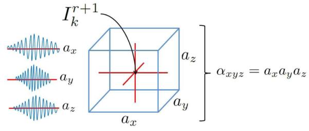
Tensor product for inphase regression coefficients. The search window surrounding point $I_k^{r+1}$ is shown. Predictor coefficients (a_x, a_y, and a_z) are calculated across each dimension. The mSLiP regression coefficients, _xyz, are tensor product of these one-dimensional coefficient vectors.

This tensor product simplifies the complexity of our regression by greatly reducing the space in which the regression is performed. Assuming that our search window has dimensions X × Y × Z, there are XY Z parameters in our predictor. By using the separable coefficient approach, we need only calculate three coefficient tensors of length X,Y , and Z, so we reduce the number our parameters calculated in our regression to X + Y + Z. For our data set, the typical reduction in the number of parameters is from 4941 to 79, thus greatly reducing the algorithm’s computational complexity.

The approach of separating the regression coefficients along each dimension of the analytic image imposes a structure on the 3D field of predictor coefficients that will be calculated. In our experiments we found that there were no visible changes in predictor accuracy and there was no measurable difference in segmentation accuracy. This preservation in accuracy can be attributed to the fact that the regression with the simplification is still flexible enough to capture the temporal coherence we wish to exploit in the RF data.

Rather than directly solving for the predictor parameters, we use an iterative method. This was done to further simplify computations and is discussed as it relates to the optimization over other algorithm parameters in Section 2.11. We use conjugate gradient descent for this optimization because we seek to solve a large number of linear equations for which conjugate gradient descent is well suited.

2.8. Segmentation Model

Segmentation is performed by maximizing the following log posterior probability with respect to the level set function, ϕ. As before, each region of the image is indexed by n = {1, 2}.

$$\begin{array}{cc}\hfill & \log p(I^1\mid I^2,\dots ,I^L,\varphi ,ϴ)\hfill \\ \hfill & \propto \sum _{k\in \Omega }H\left({\varphi }_k\right)[\sum _{r=1}^{L-1}\log p_1(I_k^{r+1}\mid I_k^r,{\alpha }_1,{\beta }_1,{\sigma }_1)\phantom{]}\hfill \\ \hfill & +\log {\Pi }_1(\mid I_k^r\mid \mid {\mu }_1,{\tau }_1)]\hfill \\ \hfill & +\sum _{k\in \Omega }(1-H({\varphi }_k\left)\right)[\sum _{r=1}^{L-1}\log p_2(I_k^{r+1}\mid I_k^r,{\alpha }_2,{\beta }_2,{\sigma }_2)\phantom{]}\hfill \\ \hfill & +\log {\Pi }_2(\mid I_k^r\mid \mid {\mu }_2,{\tau }_2)]\hfill \end{array}$$ (9)

Substituting the closed form equations for p₁, p₂, Π₁, and Π₂ then simplifying yields

$$\begin{array}{cc}\hfill & \log p(I^1\mid I^2,\dots ,I^L,\varphi ,ϴ)\hfill \\ \hfill & \propto \sum _{k\in \Omega }H\left({\varphi }_k\right)\left[\sum _{r=1}^{L-1}\left(\log \frac{{\sigma }_2}{{\sigma }_1}-\frac{e_k^{r⊺}{\stackrel{‒}{e}}_k^r}{2{\sigma }_1^2}+\frac{e_k^{r⊺}{\stackrel{‒}{e}}_k^r}{2{\sigma }_2^2}\right)\right]\hfill \\ \hfill & -\sum _{r=1}^{L-1}\left(\log \sqrt{2\pi }{\sigma }_2-\frac{e_k^{r⊺}{\stackrel{‒}{e}}_k^r}{2{\sigma }_2^2}\right)\hfill \\ \hfill & +{\lambda }_{\Pi }(\sum _{k\in \Omega }H\left({\varphi }_k\right)\left[\log \frac{{\tau }_2}{{\tau }_1}-\frac{{(\mid I_k^1\mid -{\mu }_1)}^2}{2{\tau }_1^2}+\frac{{(\mid I_k^1\mid -{\mu }_2)}^2}{2{\tau }_2^2}\right]\phantom{)}\hfill \\ \hfill & \phantom{(}-\log \sqrt{2\pi }{\tau }_2-\frac{{(\mid I_k^1\mid -{\mu }_2)}^2}{2{\tau }_2^2}),\hfill \end{array}$$ (10)

where λ_Π is a weight on the spatial magnitude term.

2.9. Priors

As in Pearlman et al. (2010) and Pearlman et al. (2011), we introduce two priors: (1) A prior that promotes the smoothness of the predictor coefficients. This prior is given by

$$\begin{array}{cc}\hfill E_S({\alpha }_1,{\beta }_1,{\alpha }_2,{\beta }_2)& =\frac{1}{2}{\alpha }_1^{⊺}{\mathbf{W}}^{⊺}\mathbf{W}{\alpha }_1+\frac{1}{2}{\alpha }_2^{⊺}{\mathbf{W}}^{⊺}\mathbf{W}{\alpha }_2\hfill \\ \hfill & \frac{1}{2}{\beta }_1^{⊺}{\mathbf{W}}^{⊺}\mathbf{W}{\beta }_1+\frac{1}{2}{\beta }_2^{⊺}{\mathbf{W}}^{⊺}\mathbf{W}{\beta }_2.\hfill \end{array}$$ (11)

where W is a first order finite difference matrix given by

$$\mathbf{W}=\left[\begin{array}{ccccccc}\hfill 1\hfill & \hfill -1\hfill & \hfill 0\hfill & \hfill 0\hfill & \hfill \cdots \hfill & \hfill 0\hfill & \hfill 0\hfill \\ \hfill 0\hfill & \hfill 1\hfill & \hfill -1\hfill & \hfill 0\hfill & \hfill \cdots \hfill & \hfill 0\hfill & \hfill 0\hfill \\ \hfill 0\hfill & \hfill 0\hfill & \hfill 1\hfill & \hfill -1\hfill & \hfill \cdots \hfill & \hfill 0\hfill & \hfill 0\hfill \\ \hfill 0\hfill & \hfill 0\hfill & \hfill 0\hfill & \hfill 1\hfill & \hfill \cdots \hfill & \hfill 0\hfill & \hfill 0\hfill \\ \hfill ⋮\hfill & \hfill ⋮\hfill & \hfill ⋮\hfill & \hfill ⋮\hfill & \hfill \ddots \hfill & \hfill ⋮\hfill & \hfill ⋮\hfill \\ \hfill 0\hfill & \hfill 0\hfill & \hfill 0\hfill & \hfill 1\hfill & \hfill 0\hfill & \hfill 1\hfill & \hfill -1\hfill \end{array}\right].$$ (12)

The finite difference matrix discretely approximates a first derivative, so E_S(α₁,β₁,α₂, β₂,) leads to first-order smoothing of the predictor coefficients. Note that this term only serves to regularize the predictor coefficients and should not directly affect the segmentation.

(2) A prior on the arc-length of the propagating front, E_AL(ϕ_k) for smoothing the segmentation, as in Chan and Vese (2001), and given by

$$E_{AL}\left({\varphi }_k\right)=\sum _{k\in \Omega }\delta \left({\varphi }_k\right)\mid \nabla {\varphi }_k\mid$$ (13)

where δ is the Dirac delta function and ▽ is the 3 × 3 × 3 discrete Laplacian.

2.10. Energy

Maximizing the likelihood is equivalent to minimizing its negative, so the overall energy is given by

$$\begin{array}{cc}\hfill E(I_k^1,\dots ,I_k^L,{\varphi }_k,ϴ)& =-\log p(I_k^1,\dots ,I_k^L,{\varphi }_k,ϴ)\hfill \\ \hfill & +{\lambda }_{AL}{E}_{AL}\left({\varphi }_k\right)+{\lambda }_S{E}_S({\alpha }_1,{\alpha }_2,{\beta }_1,{\beta }_2)\hfill \end{array}$$ (14)

where λ_S and λ_AL are weights on the smoothness priors.

2.11. Optimization

We iteratively minimize the energy functional as follows: 1) Initialize ϕ inside the blood pool. 2) Update the non-level set parameters of the model. These include the predictor coefficients, α_n and β_n, and distribution parameters σ_n, μ_n, and τ_n. 3) Update ϕ. We then iterate steps 2 and 3 until a local minimum of the energy functional is reached. The level set is updated by gradient descent, the predictor coefficients α_n and β_n are updated by conjugate gradient descent on the coefficient tensors for each dimension. Other parameters are updated by the closed form solutions:

$$\begin{array}{cc}\hfill & {\widehat{\mu }}_n=\frac{1}{N}\sum _{k=1}^N\mid I_k^1\mid ,{\widehat{\tau }}_n^2=\frac{1}{N}\sum _{k=1}^N{(\mid I_k^1\mid -{\widehat{\mu }}_n)}^2,\hfill \\ \hfill & \text{and}{\widehat{\sigma }}_n^2=\frac{1}{N}\sum _{k=1}^N{\left(e_k^r\right)}^2,\hfill \end{array}$$ (15)

where N is the number of voxels in the image.

Calculating predictor coefficients is greatly simplified by separable coefficient regression, but the regression still requires solving a very large system of equations, which is computationally burdensome to solve by inversion, so we use an iterative approach. Since we employ a Gaussian in Equation 7, the best estimator minimizes the squared error. We therefore minimize the squared residue, $e_k^{r⊺}{\stackrel{‒}{e}}_k^r$, using the conjugate gradient method. Initially setting all parameters equal, we alternately update the contour and prediction coefficients until convergence. As stated in Section 2.7, the conjugate gradient method is particularly well suited for our linear model and typically converges in just a few iterations.

3. Experiments and Results

3.1. Surgical Preparation and Ultrasound Acquisition

We obtained 27 RF sequences from 6 canines (with an average weight of 20 kg) using a Philips iE33 ultrasound imaging system (Philips Health Care, Andover, MA). Three-dimensional ECG-gated images were acquired using framerate optimization mode at sampling rates of 51-89 volumes per second. Typical image resolutions are on the order of 0.8mm in the axial direction and 1.5 mm in the lateral and elevational directions. All animal imaging studies were performed with approval of the Institutional Animal Care and Use Committee in anesthetized open-chested animals supported on mechanical ventilation. Images were acquired during brief suspensions of mechanical ventilation with an X7-2 transducer at 4.4 MHz fixed in a water bath over the heart. Time points included both baseline and one hour after surgical occlusion of the left anterior descending coronary artery. It was established in Pearlman et al. (2010) that the status of regional and global function after coronary occlusion does not affect our segmentation; thus it is not taken into account in our results. It was also shown in Pearlman et al. (2010) that SLiP worked comparably well at both end-diastole and peak systolic ejection (representing minimum and maximum average motion of the ventricle respectively), so we did not analyze the effect of image time points independently in this work. One image from each acquired cycle was segmented with the number of cycles obtained for each animal varying from 3 to 6. The images were chosen to be representative of a number of different time points in the cardiac cycle.

To exploit the temporal continuity in myocardial speckle, the search window for the coefficients of the predictor is chosen such that it encompasses distances comparable to the correlation length of the speckle. For our data this is typically on the order of 30 voxels in the axial direction and 4 voxels in each angular direction. This window is chosen by visual inspection and is fixed for all experiments. To further reduce model complexity, the number of coefficients is decimated by a factor of two in each dimension, so each coefficient represents multiple voxels.

3.2. Goals

The experiments had three goals. The first was to demonstrate that the multiframe conditional model produced accurate segmentations robust to certain image inhomogeneities, such as moderate dropout. The second was to establish how the solutions varied based on how many time points were included in the analysis. The third was to establish the algorithm’s sensitivity to varying weights on the terms in the energy functional. To this end, the new mSLiP algorithm was implemented with 2, 3, 4, and 5 frames from the cardiac sequence and compared to manual tracings of B-mode data and automated B-mode boundary detection using standard (Chan and Vese-based) level sets (Chan and Vese, 2001).

We seek to show that a region segmenter based on our temporal coherence exploiting feature is an improvement over only using B-mode intensity as a feature. A Chan-Vese method where the value at each complex voxel is represented by a circular Gaussian distribution is chosen for comparison because it assumes intensity is homogeneous over each region and only assumes a smoothness prior for the boundary. It has previously been applied for ultrasound segmentation in Angelini et al. (2004) and Yan et al. (2010). Since our goal is to show that our segmentation feature is robust to certain image inhomogeneities and produces accurate segmentations, the Chan-Vese method is also ideal for comparison because, if we remove the mSLiP segmentation feature, our method reduces to a Chan-Vese segmenter whose voxels are represented by a circular Gaussian. Thus, in comparing the two methods, we isolate only the effect of our new segmentation feature.

3.3. Advantages of the Proposed Method

Examples of the performance of the algorithms are shown on slices from the 3D data sets in figures 6, 7, 8, and 9. A typical segmentation surface is shown in Fig. 6. While the results are generated in the frustum coordinate system on analytic images, they are overlaid on the corresponding B-mode images that have been scan-line converted into Cartesian coordinates for ease of visual inspection and to present the anatomy in a familiar aspect ratio. Fig. 7 demonstrates typical cases where the Chan-Vese contours leak out through a dropout in signal intensity and mSLiP segmentations adhere to the endocardium. In all cases, the mSLiP segmentation adheres to the proper boundary. While the effect on segmentation quality is significant, these images show cases where the contour leaks out through relatively minor signal dropout. Fig. 8 demonstrates the effect of more significant dropout on the segmentation. The leftmost image in Fig. 8 contains some spurious contours resulting from the evolution of the contour. While these are rare in our experiments, they are the result of choosing the level set method and can be dealt with by tuning model parameters such as the relative weights of the arc-length prior, λ_AL, or the probability for single frame speckle, λ_Π. Fig. 9 includes a typical example that demonstrates how the segmentation results vary based on the amount of temporal information used in the analysis. In this data set, the 2-frame mSLiP still leaks through dropout, but the inclusion of more frames in the predictor prevents this. Also note that the 4-frame result is superior to the 5-frame segmentation. If enough frames are used in the analysis, the motion of the ventricle will no longer be small, thus the 5-frame segmentation begins to show a poorer result because the stationary assumption for the linear predictor has begun to break down.

Figure 6.

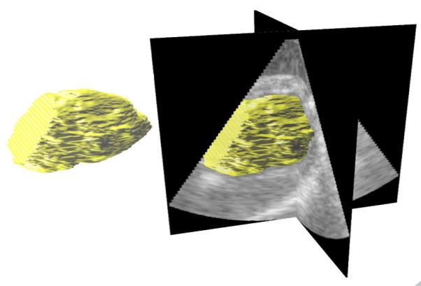
A typical segmentation surface.

Figure 7.

Slices from 3D images where Chan-Vese contours leak through moderate dropout. The lighter contour is the mSLiP result, while the darker contour is the Chan-Vese result.

Figure 8.

Slices from 3D images where Chan-Vese contours leak through significant dropout. The lighter contour is the mSLiP result, while the darker contour is the Chan-Vese result.

Figure 9.

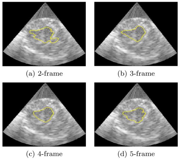
Slices from 3D images showing typical segmentations using 2,3,4, and 5 frames.

3.4. Validation and Results

The automated segmentations generated by our algorithm and the Chan-Vese approach were compared to manual tracings. Our algorithm was run on a 32-bit Windows 7 workstation with an Intel Core 2 CPU at 2.40GHz with 4.00 GB or RAM (1.00 GB reserved for the operating system). It was implemented in MATLAB and C++. The average iteration time is 1.32 minutes. The number of frames used for the predictor does not significantly effect computation time (differences are on the order of approximately 1 second). Typical solutions converge in 18 to 20 iterations.

The algorithms were quantitatively evaluated based on the following three segmentation quality indices: 1) Hausdorff distance (HD); 2) mean absolute distance (MAD), and 3) the Dice coefficient. Let A and B be two segmentation surfaces. Assume that A is generated by an automatic segmentation scheme and is the contour we wish the evaluate. B is the surface produced by manual segmentation and is our ground truth. Now, let each surface be represented by a set of points such that A = {a₁, a₂, …, a_N} and B = {b₁, b₂, …, b_M}. The MAD for surfaces A and B is defined by

$$\mathrm{MAD}(A,B)=\frac{1}{2}\left\{\frac{1}{N}\sum _{i=1}^{N}d({\mathrm{a}}_i,B)+\frac{1}{M}\sum _{j=1}^{M}d({\mathrm{b}}_j,A)\right\}$$

where $d({\mathrm{a}}_i,B)=\underset{j}{\min }\mid \mid {\mathrm{a}}_i-{\mathrm{b}}_j\mid \mid$ is the distance from point a_i to the closest point on surface B. Likewise, $d({\mathrm{b}}_j,A)=\underset{i}{\min }\mid \mid {\mathrm{b}}_j-{\mathrm{a}}_i\mid \mid$ is the distance from i point b_j to the closest point on surface A. The MAD is large when, on average, the automatic segmentation is far from the manual segmentation. The HD for surfaces A and B is defined by

$$HD(A,B)=\max \left\{\underset{i}{max}d({\mathrm{a}}_i,B),\underset{j}{max}d({\mathrm{b}}_j,A)\right\}.$$

The HD is large when individual points on the automatic segmentation surface are far from the manual segmentation surface. Unfortunately, no one metric adequately accounts for global and local distances, so both MAD and HD are necessary to evaluate the quality of a segmentation surface. Finally, let Ω_A and Ω_B be the regions enclosed by surfaces A and B, respectfully. The Dice coefficient is a symmetric similarity measure given by

$$\mathit{Dice}=\frac{2\mid {\Omega }_A\cap {\Omega }_B\mid }{\mid {\Omega }_A\mid +\Vert {\Omega }_B\mid }.$$

A value of 0 indicates that there is no overlap and a value of 1 indicates that the volumes are in perfect agreement.

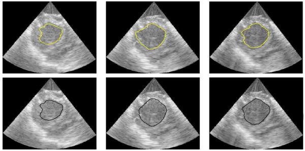
So that the surface distance measures (HD and MAD) were anatomically meaningful, all results were scan-line converted into Cartesian coordinates prior to quantitative evaluation. For visual evaluation, typical slices from segmentation surfaces along with manual tracings are shown in Fig. 10. The results of this analysis, including means and 95% confidence intervals for each quality measure, are shown in Figures 11, 12, and 13. Of particular interest for this work is the improvement in the Dice coefficient as it represents clinically relevant volume correspondence. Note that the improvement in the Dice coefficient shows diminishing returns. This is the result of the motion of the muscle as time points further from the frame being segmented are used. Similar improvements can be observed in both HD and MAD. It should be noted that, based on the confidence intervals shown in the plot, the improvement in HD is not necessarily of any significance, while the improvement in MAD tracks with the improvement in the Dice Coefficient, which can be expected since MAD represents the average distance from the correct contour and thus typically improves as volume correspondence improves.

Figure 10.

Slices from 3D images showing 4-frame mSLiP segmentations (top row) and manual tracings (bottom row).

Figure 11.

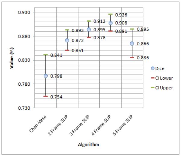
Dice Coefficient means with 95% lower and upper confidence interval.

Figure 12.

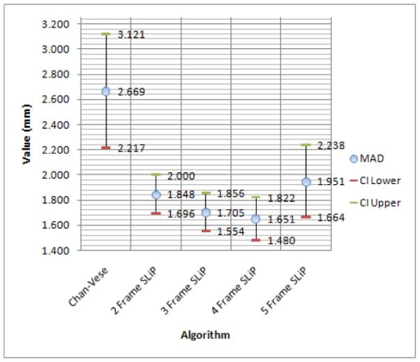
Mean Absolute Distance means with 95% lower and upper confidence interval.

Figure 13.

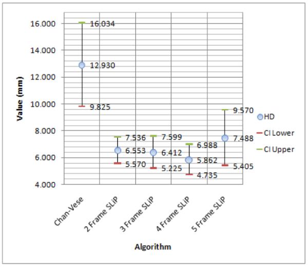
Hausdorff Distance means with 95% lower and upper confidence interval.

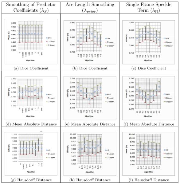
We further validate our algorithm by analyzing the sensitivity of our segmentation to changes in the weights on the three priors (i.e. linear predictor coefficient smoothing (λ_S), arc length smoothing (λprior), and the single frame speckle term (λ_Π)). We perform this analysis on a subset of our data (n=10). The results are shown in Table 1. λ_S is evaluated at 0 and then varied by factors of 10 from 0.0001 to 100. λ_S has no effect on segmentation results for any of the quality measures. This term only serves to regularize the coefficients. λprior is varied from .1 to .5 and shows a marked effect on the Dice coefficient and on MAD. Nonetheless, while these results demonstrate the value of arc length smoothing for accurate segmentation, the change in the Dice coefficient over this range is ^~5%, so the algorithm is fairly robust to λprior. λ_Π is varied from .1 to .9 and shows a similar effect on Dice and MAD values demonstrating the algorithm’s robustness to λ_Π. Nonetheless, the proper choice of λ_Π does affect segmentation accuracy.

Table 1.

Means with 95% lower and upper confidence interval of quality measures obtained by varying weights of priors. The columns correspond to λ_S, λ_prior, and λ_Π while the rows correspond to the Dice coefficient, mean absolute distance, and Hausdorff distance. (n = 10)

4. Discussion and Conclusions

We have proposed a conditional probability model for segmentation of the endocardial surface from RF echocardiography that jointly models the probability of each region based on relating the frame of interest to a subsequent sequence of frames and the complex intensities of the frame being segmented. Frames are related by means of a spatio-temporal linear predictor whose coefficients are chosen in a least squares sense based on complex speckle values. The algorithm relies solely on the signal rather than a priori knowledge of expected shape. The proposed method also utilizes temporal coherence in the data without computing expensive tracking parameters prior to segmentation. Finally, the mSLiP segmentation feature does not make a piecewise homogeneous assumption for the image and thus does not leak through boundaries that have relatively poor contrast (i.e., moderate dropout).

This approach is intended as a preprocessing step in RF phase-based speckle tracking. Because the motion of the blood is irregular, performing speckle tracking on the blood pool provides no meaningful information. The mSLiP objective function segments based on the same concept, so it is well suited for providing a geometric constraint for speckle tracking.

The key innovation of this work is the use of correlations among an ensemble of frames towards the segmentation of the endocardial surface from apex to mid-ventricle base in a single frame. This leads to more accurate estimates of predictor parameters and provides more context for the segmenter when there is prominent signal dropout. The method produced accurate segmentations and was robust to image inhomogeneities that prevent more conventional algorithms from successfully discriminating all of the endocardium. The results also show that including more temporal data in the analysis only improves the results within a small range of time points. The number of time points must be chosen such that the motion of the ventricle over the sequence is small.

Future work will focus on schemes to include more temporal data without incurring diminishing returns in segmentation results. It is also of interest to see if these methods can be extended to capture the epicardium, which is currently complicated by a difficulty in discriminating the boundary between the left ventricle and the liver (the liver also demonstrates a strong temporal coherence).

• We segment left ventricular endocardial boundaries from RF ultrasound.

• Our M.A.P. segmentation uses a joint spatial model and a multiframe conditional.

• The conditional model relates neighboring frames using a linear predictor.

• The linear predictor exploits spatio-temporal coherence in the data.

• We overcome problems due to image inhomogeneities amplified in B-mode segmentation.

References

- Angelini E, Otsuka R, Homma S, Laine A. Comparison of ventricular geometry for two real time 3d ultrasound machines with three dimensional level set. Biomedical Imaging: Nano to Macro, 2004; IEEE International Symposium on.2004. pp. 1323–1326. [Google Scholar]
- Bernard O, Touil B, D’hooge J, Friboulet D. Statistical modeling of the radio-frequency signal for partially- and fully-developed speckle based on a generalized gaussian model with application to echocardiography. Ultrasonics, Ferroelectrics and Frequency Control, IEEE Transactions on. 2007;54:2189–2194. doi: 10.1109/tuffc.2007.515. [DOI] [PubMed] [Google Scholar]
- Chan TF, Vese LA. Active contours without edges. IEEE Trans on Imag Proc. 2001;10:266–277. doi: 10.1109/83.902291. [DOI] [PubMed] [Google Scholar]
- Cremers D, Rousson M, Deriche R. A review of statistical approaches to level set segmentation: Integrating color, texture, motion and shape. International Journal of Computer Vision. 2007;72:195–215. [Google Scholar]
- Declerck J, Subsol G, Thirion JP, Subsol G, Ayache N, Ayache N, Robotique P, Epidaure P. Automatic retrieval of anatomical structures in 3d medical images. Proc. of the Conf. on Comp. Vis., Virtual Reality, and Rob. in Med; Springer-Verlag; 1995. pp. 153–162. [Google Scholar]
- Dydenko I, Friboulet D, Gorce JM, D’hooge J, Bijnens B, Magnin IE. Towards ultrasound cardiac image segmentation based on the radiofrequency signal. Med Imag Anal. 2003;7:353–367. doi: 10.1016/s1361-8415(03)00010-0. [DOI] [PubMed] [Google Scholar]
- Fundana K, Overgaard N, Heyden A. Variational segmentation of image sequences using region-based active contours and deformable shape priors. International Journal of Computer Vision. 2008;80:289–299. 10.1007/s11263-008-0160-6. [Google Scholar]
- Insana M, Meyers K, Grossman L. Handbook of Medical Imaging: Medical Image Processing and Analysis. volume 2. SPIE Press; 2000. chapter Signal Modelling for Tissue Classification; pp. 515–536. [Google Scholar]
- Langton C. Hilbert transform, analytic signal, and the complex envelope. Sig Proc and Sim News. 1999.
- Lubinski MA, Emelianov SY, O’Donnell M. Speckle tracking methods for ultrasonic elasticity imaging using short-time correlation. IEEE Trans Ultra Ferro Freq Cont. 1999;46:82–96. doi: 10.1109/58.741427. [DOI] [PubMed] [Google Scholar]
- Nillesen MM, Lopata RGP, Huisman HJ, Thijssen JM, Kapusta L, de Korte CL. 3d cardiac segmentation using temporal correlation of radio frequency ultrasound data. Proc. MICCAI. 2009;12:927–934. doi: 10.1007/978-3-642-04271-3_112. [DOI] [PubMed] [Google Scholar]
- Noble JA, Boukerroui D. Ultrasound image segmentation: a survey. IEEE Trans on Med Imag. 2006;25:987–1010. doi: 10.1109/tmi.2006.877092. [DOI] [PubMed] [Google Scholar]
- Paragios N, Deriche R. Geodesic active regions and level set methods for motion estimation and tracking. Comput. Vis. Image Underst. 2005;97:259–282. [Google Scholar]
- Pearlman PC, Tagare H, Lin B, Sinusas A, Duncan J. Segmentation of 3d echocardiography using a joint spatio-temporal predictor and signal intensity model. Proc. ISBI. 2011. To appear in.
- Pearlman PC, Tagare HD, Sinusas AJ, Duncan JS. 3d radio frequency ultrasound cardiac segmentation using a linear predictor. Proc. MICCAI. 2010;13:502–509. doi: 10.1007/978-3-642-15705-9_61. [DOI] [PMC free article] [PubMed] [Google Scholar]
- Qian X, Tagare HD. Overcoming dropout while segmenting cardiac ultrasound images. Proc. ISBI.2006. pp. 105–108. [Google Scholar]
- Shung KK, Thieme GA. Ultrasonic scattering in biological tissues. CRC Press; 1993. [Google Scholar]
- Tao Z, Tagare HD, Beaty JD. Evaluation of four probability distribution models for speckle in clinical cardiac ultrasound images. IEEE Transactions on Medical Imaging. 2006;25:1483–1491. doi: 10.1109/TMI.2006.881376. [DOI] [PubMed] [Google Scholar]
- Yan P, Jia CX, Sinusas A, Thiele K, O’Donnell M, Duncan JS. Lv segmentation through the analysis of radio frequency ultrasonic images. Proc IPMI. 2007;20:233–244. doi: 10.1007/978-3-540-73273-0_20. [DOI] [PubMed] [Google Scholar]
- Yan S, Yuan J, Hou C. Segmentation of medical ultrasound images based on level set method with edge representing mask. Advanced Computer Theory and Engineering (ICACTE), 2010 3rd International Conference on.2010. pp. V2–85–V2–88. [Google Scholar]