Figure 1.

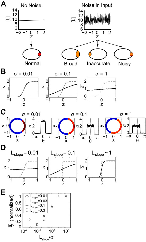
Effects of spatial noise on cell polarity. (A) Diagram showing input chemical gradient [L] without noise (left) and with noise (right) plotted against axial length z. Polarity response is represented by localization of the red species. Spatial input noise makes sensing and responding to the gradient more difficult affecting the extent, directional accuracy, and smoothness of the output polarization. (B) Spatial noise inhibits cell polarity. Increasing the magnitude of the noise (σ² = noise variance; L_slp = 0.1 μm^-1) caused a decrease in polarity of the no-positive-feedback model (NPF) in 1D simulations. The time-average of the polarity variable a (ā) with respect to z is depicted. The dashed gray line indicates response in the absence of input noise. (C) Spatial noise causes inaccurate polarization. In 2D simulations of the positive feedback model (PF), the directional accuracy was measured by comparing the response peak of polarization variable a to the direction of the input gradient. Increasing noise caused an inaccurate directional response. For each noise value, the left graph is a blue-to-red heat map representing the value of the variable a, and the right graph plots the same data as a versus the arc length θ. (D) Increasing the gradient slope (L_slp) for a fixed noise strength (σ = 0.1) improved polarization in the NPF model. The extent of polarization (ā at front) increased with steeper gradients. The dashed gray line represents the polarization in the absence of input noise. (E) Plot of polarization versus signal-to-noise ratio. For simulations of the NPF model, the y-axis represents the ā_f values normalized by subtracting 1. The x-axis represents the signal-to-noise ratio $\frac{L_{slp}}{\sigma }$ using a log-scale. Data is grouped into symbols according to L_slp values as shown by the key.