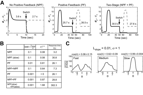
Figure 3.

Tradeoff between polarization and response time. (A) The black solid line describes time evolution of a_f, value of a at the front; the gray dashed line represents the evolution of a_b, value of a at the back. We measured the response time to an initial gradient and then switched the gradient direction. Response time is defined as the time it takes the simulation to settle to within 95% of the steady-state value. The initial gradient was applied and then after reaching steady-state, the gradient direction was switched 180^o (L_mid = 1 and L_slp = 0.01 μm^-1). Results for the NPF (left), PF (middle), and NPF+PF (right) models are shown along with the response times. The calculated settling time t_s is the average of the initial and switched response times. (B) A comparison of different model architectures in terms of polarization $\left(a_f^{norm}\right)$ and response time (t_s). For the NPF models, a larger signal-to-noise (SNR) was needed to observe polarization. In the slow versions of the models, the parameters were scaled 10-fold lower. Two-stage models are indicated by the "+" between the stages. (C) Simulations of yeast model at different speeds for the heterotrimeric G-protein cycle. The speed was normal (wild-type parameter values), 10-fold faster, and 10-fold slower. At least 20 simulations were performed and the mean value of active Cdc42 in the simulations are plotted against the angle of the cell (θ = 0 is the direction of the gradient). The mean ± SEM of cos(θ) is shown above the plot.