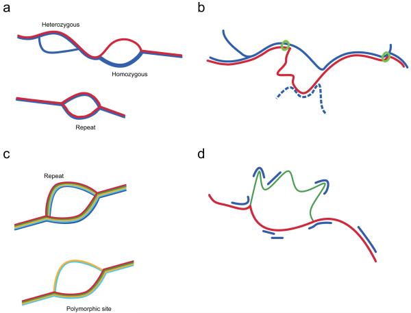
Figure 1.

Schematic representation of four methods of variation analysis using colored de Bruijn graphs; line width represents coverage. (a) Discovery of variants in a single outbred diploid individual (blue) with a reference sequence (red). True polymorphisms generate bubbles that diverge from the reference, while repeat structures lead to bubbles also observed in the reference. (b) Even when the reference allele (red) does not form a clean bubble, we can identify homozygous variant sites by tracking the divergence of the reference path from that of the sample. On finding a breakpoint, we take the longest contig in the sample (i.e. the path as far as the next junction) and ask whether the reference path returns before this point (green circle = anchoring sequence). The algorithm (path divergence) is not affected by repeat sequence within the reference allele present elsewhere in the genome of the sample (blue dotted). (c) When many samples (each in a different colour) are combined it is possible to distinguish repeat-induced bubbles (in which both sides of the bubble are present in all samples) from true variant sites (in which bubble coverage varies with genotypes and genotypes are in Hardy-Weinberg equilibrium). (d) The likelihood of any given genotype can be calculated from the coverage (blue) of each allele (green, red), accounting for contributions from other parts of the genome. In this example, the sample is heterozygous thus has coverage of both alleles, though not sufficient to enable full assembly.