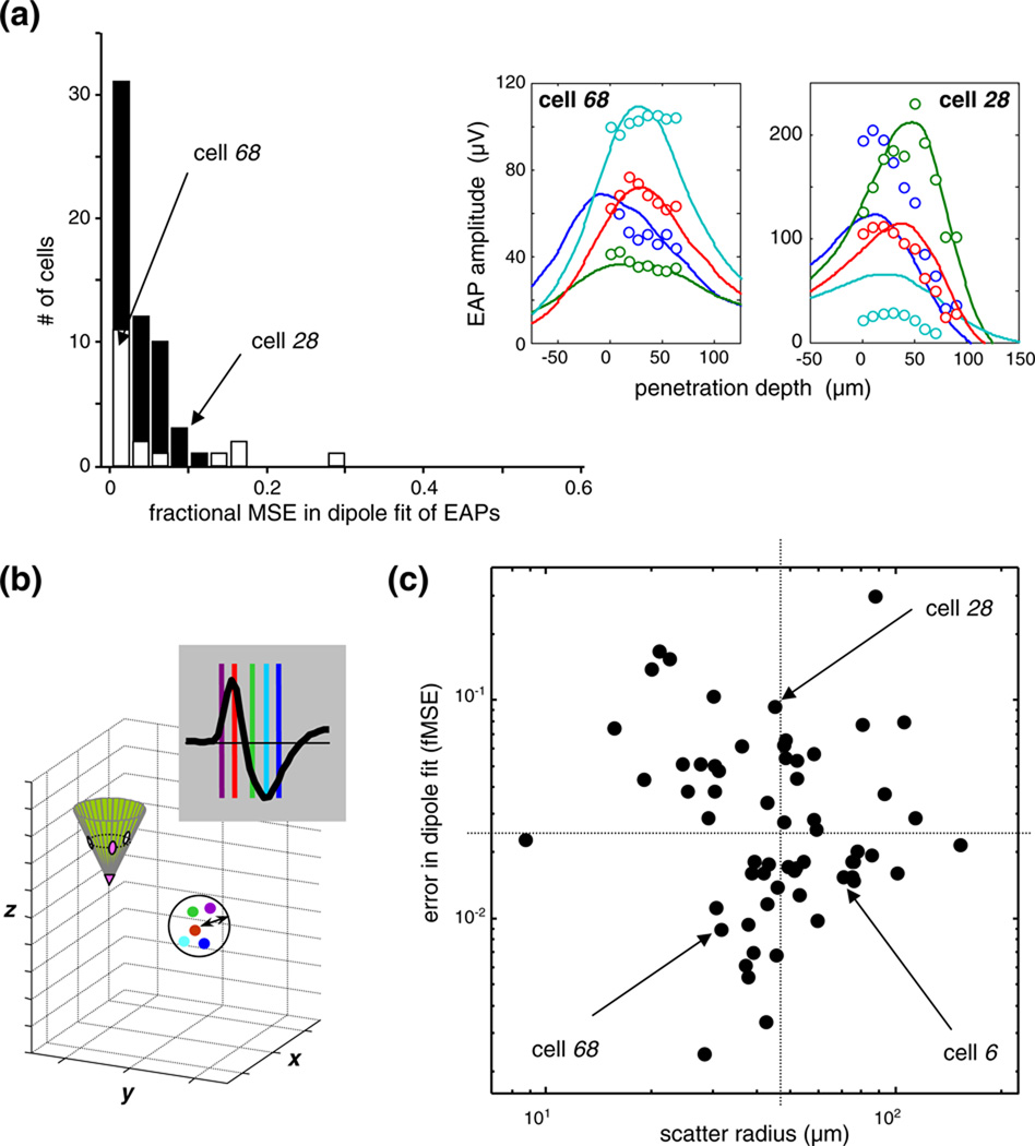
Fig. 10.

(a) The error in the optimal dipole fits. The histogram shows the sample distribution of the fractional mean-squared error, i.e., the summed squared difference between model fit and EAP data, as a fraction of the summed squared data. Histograms from the “exact-probe” cells (dark bars; N=43), to the “approximated-probe” cells (open bars; N=18) are stacked. For definition of these subsets, see Section 2. The quality of the fit and the size of the error are indicated by two examples in the insets, one with a slightly better than typical fit (cell 68; fMSE 0.009), and the other with an atypically poor fit (cell 28, fMSE 0.094). Further examples of the typical in the sample are illustrated by the 4 cells shown in Fig. 2(a); the fMSE for those cells were 0.034 for cell 4; 0.015 for cell 45; 0.039 for cell 6; 0.018 for cell 20. (b) Definition of the scatter radius—a measure of the error in dipole localization (see text for details). (c) The joint distribution, in log-log coordinates, of the fMSE error in the dipole fit (horizontal axis) and the error in dipole localization (vertical axis). Arrows indicate cells 6 (third example in Fig. 2(a)) as well as cells 28 and 68, the same two as in (a). The horizontaland vertical dotted lines indicate the sample medians. Note that the localization error (abscissa) and the fitting error (ordinate) are not correlated.