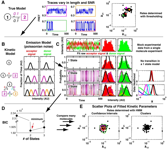
Figure 1. Workflow for SMART analysis of single molecule data.

In a typical analysis of single molecule data the distribution of rate constants determined from a simple two-state system can appear heterogeneous because of uncertainties that arise from variation in trace length and SNR. SMART addresses these limitations. Part A (left) shows a simple model used to generate 200 simulated traces, with SNR's of either 4 or 12 and trace lengths determined by a photobleaching model (see Methods). Four representative traces are shown, and the time constants for these four molecules (colors) and each of the other simulated molecules (black) determined by threshold analysis are plotted on the right. The gray star represents the inferred transition rate assuming all the molecules arose from the same population of molecules. Panels B–E show analysis of the single molecule FRET data from Panel A subject to SMART analysis. The analysis is shown for one molecule, and the data for all molecules are compared in Panel E. (B) The user specifies a set of kinetic and emission models to be fit to the observed trace. (C) Traces are analyzed individually. The donor (green) and acceptor (red) intensities are plotted as a function of time and are used directly in the fits. The cumulative histograms for the intensity of each are plotted on the right and are fit during the analysis. Fits of the models to the data are shown for the one-, two-, and three-state models of Panel B. State occupancy probabilities are shown on the left, fitted emission distributions are depicted in the middle, and the inferred transition rates between states (k _xy), and normalized likelihood values (confidence intervals) are plotted on the right (colors depict rate constants for different transitions). SMART is able to calculate confidence intervals for each of the fitted parameters. (D) The Bayesian information criterion (BIC) is used to select a model that best balances goodness of fit and the number of free parameters. The fit with the lowest Bayesian information criteria has the optimal fit. (E) Summary of data from steps (B) and (C) for the entire population of 200 molecules. The plots show different representations of uncertainties, with confidence intervals on the left (shown explicitly only for the colored traces from Panel A) and as clusters on the right (one cluster is shown). The molecules that segregated into two apparent classes by thresholding have overlapping confidence intervals (left) and fall in the same cluster (right) and thus do not provide evidence for distinct populations of molecules.