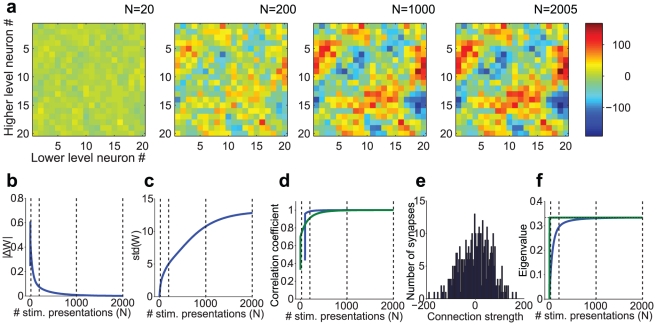
Figure 2. Example numerical implementation of the analytical results for depression-biased rSTDP learning.

a. Development of top-down synaptic weights (W) over multiple stimulus presentations. N indicates the stimulus presentation number and here we show 4 snapshots of W (N). This model had 20 lower units and 20 higher units. The strength of each synaptic weight is represented by the color in the W matrix (see scale on the right). The algorithm converged after 2005 iterations and the final W is shown on the right (see Methods for convergence criteria). b–d. Measures of weight stability and diversity. b. Norm of the change in the top-down weight matrix () as a function of stimulus presentation number N (see text). As the algorithm converges, the change in the weights becomes smaller. The dotted lines mark the iterations corresponding to the snapshots shown in part a. c. Standard deviation of the distribution of top-down weights as a function of iteration presentation number (loosely represented in the y-axis as std(W)). The final value in this plot (N = 2005) corresponds to the standard deviation of the distribution shown in part e. d. Pearson correlation coefficient between the vectorized W (N) and W(N-100) (blue line, calculated only for N> = 100) and between W(N) and the predicted value of W at the fixed point (W* = Q⁻¹; green line, see text for details). As the algorithm converges, W (N)→. e. Measure of weight diversity: Distribution of the final synaptic weights after the algorithm converged. Bin size = 4. f. Measure of absence of strong loops: Mean (blue) and maximum (green) eigenvalue of the matrix WQ, as a function of stimulus presentation number. This matrix describes the activity changes produced in a full up-down loop through the network. Eigenvalues greater than one would correspond to the existence of strong loops. The maximum eigenvalue never surpasses 0.33, which is equal to 1/. The mean eigenvalue also eventually stabilizes at this value.