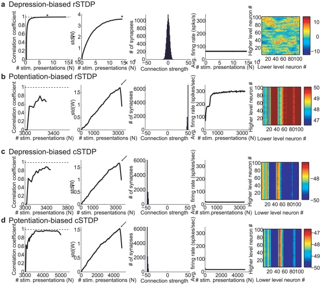
Figure 4. Representative results of integrate-and-fire simulations for different learning rules.

We consider here four possible learning rules: classical STDP (cSTDP, c,d), reverse STDP (rSTDP, a,b), depression-biased (a,c) and potentiation-based learning (b,d). For each learning rule, we show the results for a representative simulation (see summary results in Figure 5 .) The format and conventions for the subplots are the same as in Figure 3 . The subplots show the Pearson correlation coefficient between the vector containing all the entries of W (N) and that for W (N-ΔN), for ΔN = 3,000 iterations (first subplot), the standard deviation of the distribution of weights (second subplot), the distribution of weights (third subplot), the average firing rate of the lower level units (fourth subplot) and the final W. The simulation in part a converged; the convergence criteria were met at the value of N indicated by an asterisk. The simulations in b–d were classified as having “extreme weights” meaning that >50% of the weights were either at 0 or at the weight boundaries (±50). The arrows in the second subplot in b–d denote inflection points where the weights reached the boundaries and the standard deviation started to decrease. The parameters for each of these simulations are listed in the last column of Table 1 , with specifics as follows. a rSTDP,  = 1.2; b: rSTDP,  = 0.9; c: cSTDP,  = 1.2; d: cSTDP,  = 0.9. For the simulations in b–d, the weights varied most strongly across lower-level neurons, leading to the appearance of vertical bands in the final subplots (note the differences in the color scale and standard deviation values in 4b–d compared to 4a). Some lower-level neurons experienced greater joint activity than others due to the choice of Q (and hence greater plasticity); the instability of learning in these simulations then magnified these initial imbalances.