Figure 5.

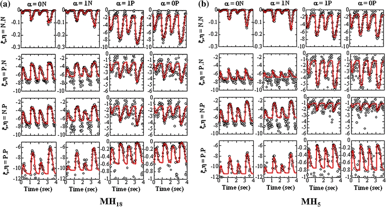
The least square fitting of the parameters. The values of \documentclass[12pt]{minimal} \usepackage{amsmath} \usepackage{wasysym} \usepackage{amsfonts} \usepackage{amssymb} \usepackage{amsbsy} \usepackage{mathrsfs} \usepackage{upgreek} \setlength{\oddsidemargin}{-69pt} \begin{document}$$ \sum {C(i)_{\xi ,\;\alpha ,\;\eta }^{\mu ,\beta ,\nu } \;{}^{IT}\langle {[ \mu ][ \beta][ \nu]} \rangle_{i} } $$\end{document} (red lines) estimated from the least square problem of Eq. (6) are compared with log W(ξ, α, η, i, IT) (circles), calculated from the MC simulation results using 10,000 samples for various combinations of the MH state (α, column) and the neighboring states (ξ and η, row). All results are from the MH₁₈ (the central unit in the filament) in the left panel and from MH₅ (near the left end of MF) in the right panel, respectively, for SL = 2.2 μm