Figure 3.
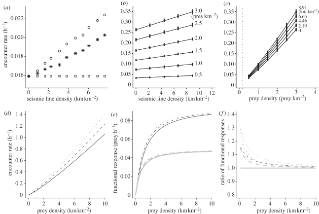
Simulated encounter rates (equations (2.1)–(2.3)) and the effect of seismic line density on the encounter rate and functional response. (a) Encounter rates for the different movement models as a function of seismic line density when prey density is fixed at 0.16 prey km−2 (squares, no response; circles, anisotropic diffusion; asterisks, anisotropic diffusion + bias). (b) Encounter rate at each prey density for the anisotropic diffusion model. Lines show the fit of the best model for encounter rate, which was the linear model in each case. (c) Encounter rate at each seismic line density for the anisotropic diffusion model. The dotted line indicates a density of 0.16 prey km−2 (compare with (a)). Lines show the fit of the best model for encounter rate, which was the power model in each case. (d) Predicted encounter rate for three seismic line densities. Encounter rate was predicted by the model C3: E = ANb + β1 Nb S, where the coefficients are A = 7.43 × 10− 2, b = 1.15 and β1 = 2.74 × 10⁻³ (solid lines, no seismic lines; dashed lines 4.46 km km−2; dotted lines, 8.91 km km−2). (e) The functional response, assuming handling times for small-bodied (black lines) and large-bodied (grey lines) prey. (f) The ratio of functional responses in landscapes with and without seismic lines, assuming handling times for small- and large-bodied prey.

