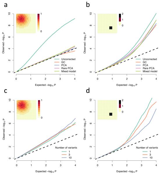
Figure 3. Comparison of methods for correcting for population structure.

(a-b) QQ plots of −log₁₀ P-values showing the uncorrected values and the values under different corrections; (c-d) Simulated rare variant load tests (Online methods); All parameters are the same as in Figure 1, except the non-genetic risk is doubled so for the Gaussian risk a and c the phenotypic mean is shifted by at most 0.8 standard deviations, while for the small, sharp risk in b and d it is shifted by at most 2 standard deviations; These are both averaged over multiple simulations in order to show the average effect. Individual experiments may vary due to the sampling variance of the trait. (a-b) averaged over 100 simulations, each testing one trait at 10,000 loci in total (10 loci on each of 1000 genealogies, representing independent genomic regions). (c-d) averaged over 10 simulations, each one testing 10,000 genealogies with either 1,3, or 10 variants in each; Abbreviations: GC, genomic control; PCA principal component analysis, using the first 10 principal components; Rare PCA, as PCA but using only variants with MAF < 4%.