Agonism/antagonism switching in allosteric ensembles

Abstract

Ligands for several transcription factors can act as agonists under some conditions and antagonists under others. The structural and molecular bases of such effects are unknown. Previously, we demonstrated how the folding of intrinsically disordered (ID) protein sequences, in particular, and population shifts, in general, could be used to mediate allosteric coupling between different functional domains, a model that has subsequently been validated in several systems. Here it is shown that population redistribution within allosteric systems can be used as a mechanism to tune protein ensembles such that a given ligand can act as both an agonist and an antagonist. Importantly, this mechanism can be robustly encoded in the ensemble, and does not require that the interactions between the ligand and the protein differ when it is acting either as an agonist or an antagonist. Instead, the effect is due to the relative probabilities of states prior to the addition of the ligand. The ensemble view of allostery that is illuminated by these studies suggests that rather than being seen as switches with fixed responses to allosteric activation, ensembles can evolve to be “functionally pluripotent,” with the capacity to up or down regulate activity in response to a stimulus. This result not only helps to explain the prevalence of intrinsic disorder in transcription factors and other cell signaling proteins, it provides important insights about the energetic ground rules governing site-to-site communication in all allosteric systems.

The paradigm that proteins acquire their function by adopting a well-defined structure has been challenged by the observation that many proteins are either intrinsically disordered (ID) under native conditions or that there is significant conformational heterogeneity within an otherwise folded protein (1–5). Of particular significance is the growing body of literature that shows allostery can be accompanied by significant changes in conformational fluctuations (6–14), and that ID sequence stretches are found in hyper-abundance in transcription factors (TFs) (5). Previously, we demonstrated that folding of intrinsic disorder can be used as a mechanism to couple binding between different functional domains (15). Our results revealed that the precise distribution of states within the native state ensemble of allosteric proteins was responsible for the magnitude of the allosteric response. In addition, the response could be modulated by tuning the ensemble through mutation or through the binding of ligands, protons, or cofactors. This model has subsequently provided insight into allosteric mechanisms in both real and designed systems (9, 16, 17). Here we address the question of whether such tuning of the ensemble can involve transforming an antagonist into an agonist (or vice versa). Answering this question will not only provide insight into allosteric mechanism (18), it could also have a broad impact on strategies currently being implemented in the development of anticancer or other agents that act by allosterically binding to their targets (19).

Most TFs have a modular structure, which includes a regulatory domain that allosterically activates or represses gene expression in response to ligand binding (20). Historically, ligands that bind to TFs have been classified by their mutually exclusive modes of action: “agonists” if they enhance gene expression or “antagonists” if they repress gene expression (19). Of interest are the cases that shatter this notion by acting as agonists under one set of conditions, and antagonists under others (21–23). In one well-documented case, Tamoxifen was developed as an antagonist of estrogen receptor (ER) and acted as such against cancer in breast tissue. However, Tamoxifen had unanticipated agonistic effects in bone and uterus tissue, resulting in patients having up to a sevenfold increase in risk for endometrial cancer (24). This phenomenon has qualitatively been explained by differing sets of binding partners that interact with ER in different tissues, yet a quantitative model describing the underlying basis of agonism/antagonism switching is lacking.

The observation that a ligand can act as an agonist and an antagonist for the same protein depending on its context is difficult to explain using the classic Monod, Wyman, Changeux [MWC] (25) or Koshland, Nemethy, and Filmer [KNF] (26) models of allostery because neither model addresses “how” binding at one site affects other sites (27) . Here we show that a general ensemble description of proteins (15) can be used to investigate agonism/antagonism switching in allosteric systems. Within the context of this model, the allosteric response of an ensemble is determined by the local equilibrium constants between high and low affinity states for different ligands, as well as the energetic coupling between the different regions. It is demonstrated, through an unbiased search of thermodynamic parameter space, that the ability to switch between agonistic and antagonistic responses for a given ligand; (i) can be robustly encoded, (ii) has simple selection rules based on the interactions between domains, and (iii) is maximized when at least one regulatory domain is either disordered or significantly populating a low affinity state. More generally, the results reveal that the ensemble allosteric model (EAM) described here and elsewhere (15) provides a vehicle for interpreting experiments and developing an understanding of the structural basis for allostery in terms of thermodynamic ground rules that govern “how” allostery works.

Results

Theory.

It is commonly recognized that multidomain regulatory proteins, such as TFs, have a modular structure and often segregate binding sites for each ligand into discrete structural domains (20, 28, 29). As such, an allosteric protein can be viewed, to a first approximation, as a group of interacting domains. This construct is completely general, with the domains being defined simply as the minimal cooperative units. Using this construct, we wish to examine whether the coupling between two domains in an allosteric protein can be affected by changes in the stability of a third domain. To accommodate this scenario, an allosteric protein will be represented as three domains that are allowed to interact with one another (Fig. 1A). Because we wish to explore the role of conformational heterogeneity in allostery, each domain will be allowed the freedom to independently exist in either a low affinity tensed (T) state or a high affinity relaxed (R) state, resulting in eight possible microstates (i.e., TTT, RTT, TRT, TTR, TRR, RTR, RRT, and RRR), representing all possible combinations of having each domain either in T or R. In the case of ID proteins, the T state would correspond to the unfolded (U) state and the R would correspond to the folded (F) state for each domain. The important feature of this model, which is the reason why each domain can “sense” the other domains, is that the free energy of any microstate relative to the reference state (i.e., RRR) is composed of the free energy of undergoing an R to T transition in any domain (ΔG_i), plus the free energy of breaking the interaction (Δg_int ,i-j) between the R states for the two domains in question. For this system the partition function, which is simply the sum of the statistical weights (S_i) of all microstates, is;

[1A]

which, when written in expanded form using the expressions in Fig. 1B, gives:

[1B]

Fig. 1.

Three-domain allosteric protein. (A) Schematic representation of a three-domain allosteric protein comprised of domains I, II, and III that can bind ligands A, B, and C, respectively. Each domain is coupled to the other two domains through an interaction energy (Δg_int ,i-j), which is schematically represented as a shaded area between domains. (B) Free energy contributions, Boltzmann statistical weights (S_i), and probabilities of each microstate in the ensemble (Note: K_i = Exp[-ΔG_i/RT] and ϕ_i-j = Exp[-Δg_int ,i-j/RT]). Each microstate represented in the left column is either completely high-affinity (RRR), partially high-affinity (TRR, RTR, RRT, RTT, TRT, TTR), or completely low-affinity (TTT). The free energy contributions come from the transition of each domain to the low-affinity T state () plus the energy of breaking the interactions between domains (). Note: For presentation purposes only, the T states for each domain are depicted as being disordered. In reality, both T and R can be folded and competent to bind ligand. The only requirement is that one of those states (by convention, R) binds ligand with higher affinity. (C) A specific case demonstrating an agonistic allosteric response. Shown are microstates that are significantly populated (i.e., > 3%) before (Left) and after (Right) the addition of ligand A. In the absence of ligand A, the summed probability of microstates with domain III in the R state (i.e., the active microstates—domain III colored yellow) are only marginally populated (approximately 20%). Upon addition of ligand A, redistribution of the ensemble results in a positive shift in the population of these microstates (approximately 73% = 43%+30%), which corresponds to an agonistic response (i.e.,CR_III,A = +0.06). The parameters used are ΔG₁ = -1.7, ΔG₂ = 2.0, ΔG₃ = -0.9, Δg₁₂ = -2.3, Δg₂₃ = 0.1, Δg₁₃ = 1.5, and Δg_Lig,A = -5.0 all in kcal/mol. (D) A specific case demonstrating an antagonistic allosteric response. Unlike the case of agonism, the active microstates are significantly populated in the absence of ligand A (approximately 95% = 89%+6%). Upon addition of ligand A, redistribution of the ensemble results in a negative shift in the population of these microstates (35%), which corresponds to an antagonistic response (i.e.,CR_III,A = -0.06). The parameters used are ΔG₁ = -2.1, ΔG₂ = 1.0, ΔG₃ = 1.2, Δg₁₂ = -1.7, Δg₂₃ = 0.6, Δg₁₃ = -2.7, and Δg_Lig,A = -5.0, all in kcal/mol.

Examination of this expression reveals that coupling between domains results when there is a nonzero interaction energy between domains i and j (i.e., Δg_int ,i-j ≠ 0 or ϕ_i-j ≠ 1). When the interaction energy is positive (i.e., Δg_int ,i-j > 0 or ϕ_i-j < 1), it is unfavorable to break the interaction between the R states of each domain. This situation would exist, for example, when hydrophobic surfaces are excluded from interacting with solvent. In the case where Δg_int ,i-j < 0 (i.e., ϕ_i-j > 1), it is energetically favorable to break the interaction and to have the surfaces interact with solvent. In the case where Δg_int ,i-j = 0 (i.e., ϕ_i-j = 1), the domains are thermodynamically independent and behave as if they are simply tethered. As discussed below, the magnitude and the sign of the interaction energies significantly affects the apparent coupling between domains.

To explore the extent of coupling, perturbations to each domain can be made and the effect of the perturbation on the other domains can be monitored. For the case being investigated here, we are interested in the allosteric response of one domain to the binding of a ligand in one or both of the other domains. To accommodate this scenario, we introduce binding sites for three different ligands such that domains I, II, and III in Fig. 1 are depicted as having binding sites for ligands A, B, and C, respectively. We are interested in the extent to which the binding of ligand A to domain I can influence the binding of ligand C to domain III, and we wish to know to what extent does binding of ligand B to domain II influence the observed coupling between domains I and III.

Straightforward linkage principles (30) dictate that the introduction of a ligand will result in preferential binding to the microstate with the highest affinity, and thus a redistribution of the ensemble to favor those microstates with high affinity. To capture this effect, the binding of the respective ligands in Fig. 1 is facilitated through the R state for each domain, which is considered to be the high affinity state. Thus, microstates RRR, RTT, RRT, and RTR can bind ligand A, microstates RRR, TRT, RRT, and TRR can bind ligand B, and microstates RRR, TTR, RTR, and TRR can bind ligand C, as in each case the domain that binds the specific ligand in question is in the R state (Fig. 1B). In the case of binding to ligand A, the partition function in the presence of ligand becomes;

[2]

where Z_Lig,A = (1 + K_a,A[A]), and K_a,A is the intrinsic association constant of the R state of domain I for ligand A. Inspection of Eq. 2 reveals that microstates that are competent to bind ligand A are stabilized by Δg_Lig,A = -RT ln(Z_Lig,A) = -RT ln(1 + K_a,A[A]). Of course at [A] ≪ 1/K_a,A, Eq. 2 reduces to Eq. 1. Note that of the four microstates wherein domain III is in the R state (i.e., RRR, RTR, TRR, and TTR), only two (i.e., RRR and RTR) are directly affected by ligand A. To determine the impact of ligand A on the ability of domain III to bind ligand C, we need only compare expressions for the probability of domain III to be in the R state, both with and without ligand A;without ligand A;

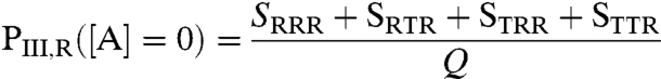[3]

with ligand A;

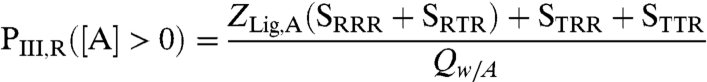[4]

As the expressions reveal, the effect of ligand A on the probability of microstates that can bind ligand C will depend on the statistical weights of the different microstates in the ensemble, which in turn will depend on the intrinsic stabilities of each domain and the interaction energies between domains (see Fig. 1B). To quantify the effect, we previously introduced the coupling response (15), which is a measure of the sensitivity of the population of microstates that can bind ligand C to the addition of ligand A;

[5]

where CR_III,A is the sensitivity of domain III to the binding of ligand A. The sign of the CR_III,A determines whether ligand A is an agonist or an antagonist; if CR_III,A is positive, ligand A is an agonist because addition of ligand A will stabilize the high affinity R state of domain III and thus increase the affinity for ligand C. Conversely, if CR_III,A is negative, ligand A is an antagonist. In actuality, most parameter combinations produce minimal coupling between domains. However, there exist multiple parameter sets that result in significant coupling that is either agonistic (Fig. 1C) or antagonistic (Fig. 1D) (15), and the hallmark feature of these parameter combinations is that the coupling is maximized when one or both domains are poised at the thermodynamic transition between the T and R states of the different domains. In the case of ID proteins, wherein the T state is unfolded, the equilibrium is poised such that one or a number of domains are significantly (approximately 95%) disordered (15).

For the current study, we are interested in the impact of the binding of a second ligand (to a separate domain) on the coupling response, as described above. To account for this effect, we need only introduce the impact of the binding of ligand B (to domain II) on the probability of domain III to be in the R state, both with and without ligand A (similar to Eqs. 3 and 4). With ligand B and without ligand A, the expression is:

[6]

where Z_Lig,B is analogous to Z_Lig,A and Q_w/B is similar to Q_w/A (Eq. 2), except that in the case of ligand B, only microstates wherein domain II is in the R state (i.e., RRR, RRT, TRR, and TRT) are affected. With both ligands A and B, the probability of domain III to be in the R state becomes:

[7]

The coupling response [Eq. 5] in the presence of ligand B thus becomes;

[8]

which, like Eq. 5, provides a measure of how the binding of ligand A to domain I influences the probability of domain III to be in the R state, except that in this case ligand B is also present. We wish to know whether ligand B can convert ligand A from an agonist to an antagonist (or vice versa).

Results of the Model.

Transcription factors, and indeed most allosteric proteins, are considered to be either positive or negative regulators of the functions they control. It therefore might be expected that parameter combinations that are numerically close in value (i.e., stabilities and interaction energies are similar), would exhibit the same phenomenological response, being either agonistic or antagonistic, but not both. Interestingly, such a conclusion is not borne out of the current analysis. Shown in Fig. 2 is one example of quantitatively identical parameter combinations that nonetheless produce opposite allosteric effects. For the parameter combinations noted, the energy landscape of the ensemble in the absence of ligand B is depicted in Fig. 2A. As shown, the ensemble is dominated by the completely T state (i.e., TTT) prior to the addition of ligand A (Fig. 2A, Right). Upon addition of ligand A, microstates with domain I in the R state are stabilized by the amount Δg_Lig,A (Fig. 2A, Left, red bars). This redistributes the ensemble, shifting the populations of all microstates such that there is an increase in the probability of domain III to be in the R state (Fig. 2A, Right). This leads to a macroscopic agonistic response to ligand A (ΔP_III,R = 51%-3% = +48%).

Fig. 2.

Specific thermodynamic architectures can produce agonism/antagonism switching. Example of a thermodynamic architecture that produces agonism-antagonism switching: ΔG₁ = -6.75, ΔG_2,B=0(1) = -4.4, ΔG_2,B>0(2) = 0.6, ΔG₃ = -2.7, Δg₁₂ = 6.8, Δg₂₃ = 4.8, Δg₁₃ = -1.9, and Δg_Lig,A = -5.0 kcal/mol. Individual free energies and populations for each microstate showing an (A) agonistic and (B) antagonistic response. Shown for both cases (Left) are the free energies of each microstate in the absence (blue bars) and presence (red bars) of ligand A (depicted as blue circles). Shown also for each case are the populations of microstates in the absence (Right, Top) and the presence (Right, Bottom) of ligand A. For the case of agonism (A), the summed population of microstates with domain III in the R state rises from 3% to 51%, while for antagonism (B) those microstates decrease from 94% to 58%. C. Coupling response (CR) dependence on stability of domains I and II (holding all other variables constant). Position 1 (yellow circle at local maximum) exhibits agonistic response to ligand A in the absence of ligand B. Position 2 (yellow circle at local minimum) exhibits antagonistic response to ligand A in the presence of ligand B (Δg_Lig,B = -5.0kcal/mol).

The converse situation occurs in Fig. 2B, which depicts the energy landscape of the ensemble in the presence of ligand B. The microstates with domain II in the R state are now lower in energy relative to the situation without ligand B (Fig. 2A, Left), leaving the ensemble poised to respond in a different manner (Fig. 2B, Right). In this case, the addition of ligand A will still stabilize states with domain I in the R state as before (Fig. 2B, Left, red bars). In this case, however, redistribution reveals an antagonistic relationship between ligand A and the R state of domain III (ΔP_III,R = 58%-93% = -35%, Fig. 2B, Right). The results are summarized in Fig. 2C, where the dependence of the allosteric response on the stabilities of domains I and II is shown (all other parameters are constant). Clearly visible is the fact that within a range of stabilities for domain I, the sign of the allosteric response to ligand A can be modulated simply by tuning the stability of domain II. For the case examined here, the tuning of the stability of domain II is facilitated through the binding of a ligand. In reality, however, the conversion can also be facilitated by mutations, covalent modification or changes in pH. The importance of the result is that it demonstrates how a single thermodynamic architecture, within the framework of the most simple three-domain model, can poise the energy landscape to respond in a “functionally pluripotent” manner. All that is required to transform an agonist to an antagonist (or vice versa) is the presence of a second ligand that binds to a distinct regulatory site. We note that although the results presented here were generated using only one value for the binding energies for Ligands A and B (i.e., Δg_Lig,A = Δg_Lig,B = -RT ln(1 + K_a[X]) = -5.0 kcal/mol), varying either or both parameters does not qualitatively change the results [SI Appendix (1)].

Thermodynamic Basis for Agonism/Antagonism Switching.

To determine the generality of the agonism-antagonism switching result shown in Fig. 2, and to investigate the determinants of the switching, we performed an unbiased search of parameter space by systematically exploring all possible combinations of values for ΔG₁, ΔG₂, ΔG₃, Δg_int ,1–2, Δg_int ,1–3, and Δg_int ,2–3 that produced such results [SI Appendix (2)]. Surprisingly, parameter combinations that produced agonism/antagonism switching were highly degenerate. The stability of any particular domain or interaction energy was not critical to ensure switching potential. Nonetheless, closer inspection of the data reveals that the organizing principles for agonism/antagonism switching center on the sign of the interaction energies between the domains. Shown in Fig. 3A is a volume plot of the interaction energies (Δg_int ,i-j) showing the parameter combinations that produce optimum agonism/antagonism switching. Of note is that there are four nodes of parameter combinations (Fig. 3A, blue). Remarkably, this plot reveals that the thermodynamic “ground rules” conferring the ability to switch responses, within the framework of the three-domain ensemble model, have two simple interaction architectures: either one or all three interaction energies (Δg_int ,i-j) must be negative (Note: −++ corresponds to Δg_int ,1–2, < 0, Δg_int ,2–3 > 0 and Δg_int ,1–3 > 0). In contrast, the nodes that represent either one or all three interaction energies (Δg_int ,i–j) being positive (Fig. 3A, gray) are not competent to switch.

Fig. 3.

Energetic rules for agonism-antagonism switching. (A) Plot of interaction parameters (i.e., Δg₁₂, Δg₂₃, and Δg₁₃) that exhibit significant agonistic (> 35%) and antagonistic (< -35%) responses within a single architecture (blue nodes labeled 1–4). Each node is represented by three + or − signs that correspond to the sign of the coupling energies, Δg₁₂, Δg₂₃, and Δg₁₃, respectively. For contrast, parameter combinations that do not exhibit switching are shaded in gray (See text for details). (B) Schematic representation of the allosteric interdomain coupling for each of the switch-competent nodes in (A) with each node numbered and represented by three + or −. Red and blue arrows indicate an antagonistic and an agonistic relationship between two domains, respectively. The red and blue arrow indicates that domain III is impacted both positively and negatively through the direct and indirect effects, as described in text. Note: The color of the arrows connecting domains II and III refer to the overall impact on domain III from stabilization of domain I. For example, in Node 3 stabilization of domain I destabilizes domain II (making the arrow red). However, that destabilization of domain II (because of negative coupling to domain III) has the effect of stabilizing domain III (making the arrow to domain III blue). (C) Schematic representation of the allosteric interdomain coupling for each of the switch-incompetent nodes in (A). The coloring scheme is similar to (B) and demonstrates that switch-incompetent architectures produce either committed agonists (+++, −−+) or committed antagonists (+−−, −+−) because the direct and indirect effects are of the same sign.

Inspection of the ensemble thermodynamic architecture reveals the underlying basis for why some parameter combinations are competent to facilitate switching while others are not. For the case of switching-competent architectures, the stabilization of domain I through the binding of ligand A will have the net effect of destabilizing domains for which the interaction energy is negative and stabilizing domains for which interaction energy is positive. For instance, consider Node 1 in Fig. 3A, wherein, domains I and III are negatively coupled, but the other coupling energies are positive. Addition of ligand A will stabilize domain I, which will antagonistically affect domain III in a manner similar to the example in Fig. 1D. However, since the two remaining interaction energies are positive, stabilization of domain I will also agonistically affect domain II, which in turn, will agonistically affect domain III. As a result, the binding of ligand A has two different and opposing effects on domain III. The overall observed effect that is manifested at domain III is the result of an energetic competition between the “direct” interactions of domains I and III (Fig. 3B, Node 1, red arrow) and the “indirect” interactions of domain I and III (i.e., those which are mediated through domain II) (Fig. 3B, Node 1, blue arrows). Depending on the magnitudes of the positive and negative effects, different responses can prevail. Addition of ligand B simply changes the relative contribution of the indirect impact relative to the direct impact. Interestingly, in some cases addition of ligand B converts an agonist to an antagonist, while in other cases, ligand B converts an antagonist to an agonist.

In contrast to the switch-competent architectures (Fig. 3B), the parameter combinations that result in switch-incompetent architectures (Fig. 3A, gray) do not produce opposing energetic effects through the direct and the indirect interactions. In these cases, ligand A is either a committed agonist (Fig. 3C, Left) or a committed antagonist (Fig. 3C, Right) because in both cases the direct impact of ligand A is the same sign as the indirect impact. Addition of ligand B simply reinforces the energetic relationship that existed in the absence of ligand B. Thus, the ability for allosteric proteins to facilitate agonism/antagonism switching is robustly encoded in the energy landscape, being possible even in the simplest possible architectures that can account for binding at three sites. This point is especially noteworthy considering that allosteric effects in most systems are often sensitive to changes in a second ligand (e.g., pH, salt, etc.), indicating that they possess, in principle, the minimum level of complexity required to potentiate switching.

Further insight into the origins of the four nodes shown in Fig. 3A can be gained by recasting the energetic parameter combinations in terms of the probability of domains I and II to be in the R state in the absence of ligand (i.e., P_I,R and P_II,R). Shown in Fig. 4 are the parameter combinations that produce ΔP_III,R values in excess of +/-20% (yellow), +/-30% (orange) and +/-40% (red). Several features stand out. First, there are two regions that maximize the switching behavior, and these regions correspond to cases where either one or both of the regulatory domains (i.e., domains I and II) are populating the T state a significant fraction of time in the absence of ligands (Fig. 4, dashed boxes). In the case of ID proteins, this scenario would correspond to being intrinsically disordered (ID) a substantial fraction of the time. Second, there is an asymmetry in the plot. Although Region 1 shows a more degenerate set of combinations of P_I,R and P_II,R that can facilitate the significant switching potentials (i.e. the spread in the points is greater around Region 1 than Region 2), the point density in Region 2 is threefold higher for architectures wherein two domains are disordered [SI Appendix (3)]. For ID proteins this result would mean that switching-competent proteins are perhaps more likely to have two different disordered domains. Put another way, sequence segments that are identified as ID may actually be comprised of multiple, thermodynamically (and/or functionally) distinct, domains. Although speculative, this notion is supported by the observed differential activity of glucocorticoid receptor isoforms that differ in the length of their disordered N-terminal domains (23). In any case, the analysis clearly shows that for systems, which are competent to switch between agonism and antagonism, the ensemble equilibria must be poised at a point where the system is maximally able to respond to both ligands.

Fig. 4.

Switching-competence is maximized when regulatory domains are predominantly populating low affinity or ID states. Plot of the probability of domain I being in the R state (i.e., P_I,R = P_RRR + P_RTR + P_RRT + P_RTT) vs. probability of domain II being in the R state (i.e. P_II,R = P_RRR + P_TRR + P_RRT + P_TRT) in the absence of ligand for switching-competent architectures. Colors indicate the magnitude of the change in probability for agonist and antagonist switching: yellow (± 20%), orange (± 30%), and red (± 40%); i.e., the architecture must exhibit an agonistic and an antagonistic response from ligand A exceeding the positive and negative thresholds in the absence and presence of ligand B (or vice versa). Maximum switching responses (dashed boxes) are observed in two regions, where either domain I only (i.e., Region 1) or both domains I and II (i.e. Region 2) are predominantly populating the T state (or in the case of ID proteins, the unfolded (U) state).

Implications of the Model.

The significance of the results presented in Figs. 2–4 are threefold. First, they demonstrate that agonism/antagonism switching can be robustly encoded in the energy landscape of a protein. Second, they reveal that the same ensemble-based model of allostery that can explain the effects of interconversion between U and F states in ID proteins (15), describes equally well the effects of conformational interconversion between two ostensibly folded conformations, both of which may bind ligand, albeit with different affinities (i.e., T and R), as described here. Third and most important, the results directly undermine the (visually appealing) notion of an obligatory allosteric pathway that mediates coupling between sites. As Fig. 2 demonstrates, the overall allosteric effect is a manifestation of the precise balance of energies in the protein, energies that can be modulated (in analog fashion) through the titration with ligands, salts, or pH. While from Fig. 3 it is clear that the energies from direct (i.e., domain I to domain III) and indirect (i.e., domain I to domain III, via domain II) contributions to the coupling should be experimentally attainable for real systems (an endeavor that, based on the results presented here, would be a logical course of action), the notion that the resultant energies can be ascribed to structural pathways between those domains is unfounded. Because the coupling is determined by intrinsic stabilities and interaction energies between each domain, any mutation that perturbs the stability will impact the coupling, regardless of whether there are changes to the interior of (or the path through) the protein. Toward this point, it has been demonstrated that surface Val to Gly mutations, which perturb the local conformational equilibrium, can have long range effects, even in the absence of changes to the average structure (31, 32). Such experimental results are important because they validate the tenets of the model presented here, and help to reconcile the observations that allosteric coupling; (i) can occur in the absence of a pathway of structural and dynamic changes linking the two sites (7, 11), (ii) can occur in the absence of structural changes at all (8, 12, 31, 33), and (iii) can be correlated to stability changes in different parts of the protein (34). Such observations are difficult to reconcile in terms of obligatory allosteric pathways through the protein, but are readily reconcilable in the context of the model presented here.

Relationship to Classical Models of Allostery.

The allosteric model presented here differs from the classic MWC (25) and KNF (26) models. The fundamental premise of MWC is that the different sites are coupled through two quaternary conformations, both of which can bind ligand. The apparent cooperativity in MWC results from a ligand driven shift from the low affinity T state to the high affinity R state. Importantly, the MWC formulation explicitly treats neither the interactions between domains nor the individual conformational equilibria describing the relative populations of T and R for each domain. The KNF model, on the other hand, does explicitly consider the interaction between domains, but that interaction is obligatorily coupled to the binding of the ligand. As such, like the MWC, the impact of the preexisting local conformational equilibria is not considered in the KNF model. This is the quintessential difference between the ensemble allosteric model (EAM) (15, 35) as defined here and the classic MWC and KNF formulations. By explicitly considering the (microscopic) conformational equilibria within the different functional domains, as well as the coupling of those processes, the EAM provides information that previous models do not—the underlying thermodynamic ground rules that relate allosteric coupling to the energetics of the local cooperative substructures in the protein. The importance of these ground rules is that they provide a framework for understanding the complex interplay between structure, dynamics (i.e., conformational heterogeneity) and function, a framework that provides general insight into “how allostery works.”

Conclusions

The results presented here reveal a new dimension to allostery. Ligands for allosteric proteins have typically been viewed as either agonists or antagonists for a given function, depending on whether the activity is enhanced or repressed. Anecdotal evidence has emerged, however, that has called into question this classic view. Some allosteric effectors have been shown to be agonistic under some conditions, and antagonistic under others (21–23), although the molecular basis of this duality is not known. The results presented here reveal that even in the context of the most simple three-domain architecture, protein ensembles can evolve with the capacity to respond to a ligand both agonistically and antagonistically, with the determining factor being how much of a second allosteric effector is present. In essence, rather than being considered as molecular switches with fixed responses to a particular ligand, many allosteric proteins may in fact have evolved to be “functionally pluripotent” with the ability to up or down regulate activity depending on the physiological circumstances.

Interestingly, and perhaps counterintuitively, agonism/antagonism switching does not require that the nature of the interaction between the ligand and its binding site be different. Indeed, in the context of the model presented here, all binding (whether it produces agonism or antagonism) is facilitated by the R state of the domain (which corresponds to an equivalence of structure), a notion that is difficult to reconcile in terms of models that rely on a mechanical pathway to understand allostery. Instead, the determining factor for whether binding produces agonism or antagonism is the stabilities of the microstates in the ensemble (which is determined by the sign and magnitude of the domain stabilities and coupling energies). Perhaps the most surprising result, and the reason why agonism/antagonism switching is even possible, is the observation that systems that are close in energetic parameter space can produce opposite phenomenological responses. This reality, as well as the significant degeneracy of potential parameter combinations that can facilitate switching, provides allosteric proteins with a robust repertoire of potential regulatory strategies.

The potential benefits of pluripotent allostery, as defined here, are compelling and perhaps can explain why, for instance, transcription factors “turn on” various target genes to different degrees (36). Can the binding to a subset of DNA sequences actually repress transcription of some genes? The importance of answering this question and others like it is not just academic. It is well known that disregulation of many members of the steroid hormone receptor (SHR) family of transcription factors (e.g., estrogen, androgen, progesterone, and glucocorticoid receptors) are associated with cancers in various tissues (37). Understanding how elevated or depressed concentrations, splicing variants, isoforms and/or mutations affect the allosteric communication in SHRs may be the key to deciphering their role in cancer, and to developing appropriate intervention strategies.

References

- 1.Wright PE, Dyson JH. Intrinsically unstructured proteins: Re-assessing the protein structure-function paradigm. J Mol Biol. 1999;293:321–331. doi: 10.1006/jmbi.1999.3110. [DOI] [PubMed] [Google Scholar]
- 2.Uversky VU, Oldfiend CJ, Dunker AK. Showing your ID: intrinsic disorder as an Id for recognition, regulation and cell signaling. J Mol Recognit. 2005;18:343–384. doi: 10.1002/jmr.747. [DOI] [PubMed] [Google Scholar]
- 3.Dunker AK, et al. Intrinsically disordered protein. J Mol Graph Model. 2001;19:26–59. doi: 10.1016/s1093-3263(00)00138-8. [DOI] [PubMed] [Google Scholar]
- 4.Babu MM, Lee R, de Groot NS, Gsponer J. Intrinsically disordered proteins: Regulation and disease. Curr Opin Struc Biol. 2011;21:432–440. doi: 10.1016/j.sbi.2011.03.011. [DOI] [PubMed] [Google Scholar]
- 5.Liu J, et al. Intrinsic disorder in transcription factors. Biochemistry. 2006;45:6873–6888. doi: 10.1021/bi0602718. [DOI] [PMC free article] [PubMed] [Google Scholar]
- 6.Bai F, et al. Conformational spread as a mechanism for cooperativity in the bacterial flagellar switch. Science. 2010;327:685–689. doi: 10.1126/science.1182105. [DOI] [PubMed] [Google Scholar]
- 7.Clarkson MW, Gilmore SA, Edgell MH, Lee AL. Dynamic coupling and allosteric behavior in a nonallosteric protein. Biochemistry. 2006;45:7693–7699. doi: 10.1021/bi060652l. [DOI] [PMC free article] [PubMed] [Google Scholar]
- 8.Cooper A, Dryden DT. Allostery without conformational change. A plausible model. Eur Biophys J. 1984;11:103–109. doi: 10.1007/BF00276625. [DOI] [PubMed] [Google Scholar]
- 9.Freiburger LA, et al. Competing allosteric mechanisms modulate substrate binding in a dimeric enzyme. Nat Struct Mol Biol. 2011;18:288–294. doi: 10.1038/nsmb.1978. [DOI] [PMC free article] [PubMed] [Google Scholar]
- 10.Laine O, Streaker ED, Nabavi M, Fenselau CC, Beckett D. Allosteric signaling in the biotin repressor occurs via local folding coupled to global dampening of protein dynamics. J Mol Biol. 2008;381:89–101. doi: 10.1016/j.jmb.2008.05.018. [DOI] [PMC free article] [PubMed] [Google Scholar]
- 11.Pan H, Lee JC, Hilser VJ. Binding sites in Escherichia coli dihydrofolate reductase communicate by modulating the conformational ensemble. Proc Natl Acad Sci USA. 2000;97:12020–12025. doi: 10.1073/pnas.220240297. [DOI] [PMC free article] [PubMed] [Google Scholar]
- 12.Popovych N, Sun S, Ebright RH, Kalodimos CG. Dynamically driven protein allostery. Nat Struct Mol Biol. 2006;13:831–838. doi: 10.1038/nsmb1132. [DOI] [PMC free article] [PubMed] [Google Scholar]
- 13.Reichheld SE, Yu Z, Davidson AR. The induction of folding cooperativity by ligand binding drives the allosteric response of tetracycline repressor. Proc Natl Acad Sci USA. 2009;106:22263–22268. doi: 10.1073/pnas.0911566106. [DOI] [PMC free article] [PubMed] [Google Scholar]
- 14.Smock RG, Gierasch LM. Sending signals dynamically. Science. 2009;324(5924):198–203. doi: 10.1126/science.1169377. [DOI] [PMC free article] [PubMed] [Google Scholar]
- 15.Hilser VJ, Thompson EB. Intrinsic disorder as a mechanism to optimize allosteric coupling in proteins. Proc Natl Acad Sci USA. 2007;104:8311–8315. doi: 10.1073/pnas.0700329104. [DOI] [PMC free article] [PubMed] [Google Scholar]
- 16.Stratton MM, Loh SN. On the mechanism of protein fold-switching by a molecular sensor. Proteins. 2010;78:3260–3269. doi: 10.1002/prot.22833. [DOI] [PMC free article] [PubMed] [Google Scholar]
- 17.Garza AS, Khan SH, Moure CM, Edwards DP, Kumar R. Binding-folding induced regulation of AF1 transactivation domain of the glucocorticoid receptor by a cofactor that binds to its DNA binding domain. PLoS ONE . 2011;6:e25875. doi: 10.1371/journal.pone.0025875. [DOI] [PMC free article] [PubMed] [Google Scholar]
- 18.Kenakin TP. ‘7TM receptor allostery: Putting numbers to shapeshifting proteins. Trends Pharmacol Sci. 2009;30:460–469. doi: 10.1016/j.tips.2009.06.007. [DOI] [PubMed] [Google Scholar]
- 19.Kenakin T, Miller LJ. Seven transmembrane receptors as shapeshifting proteins: The impact of allosteric modulation and functional selectivity on new drug discovery. Pharmacol Rev. 2010;62:265–304. doi: 10.1124/pr.108.000992. [DOI] [PMC free article] [PubMed] [Google Scholar]
- 20.Latchman DS. Transcription factors: An overview. Int J Biochem Cell B. 1997;29:1305–1312. doi: 10.1016/s1357-2725(97)00085-x. [DOI] [PubMed] [Google Scholar]
- 21.Hol T, Cox MB, Bryant HU, Draper MW. Selective estrogen receptor modulators and postmenopausal women’s health. J Womens Health. 1997;6:523–531. doi: 10.1089/jwh.1997.6.523. [DOI] [PubMed] [Google Scholar]
- 22.Katzenellenbogen BS, Montano MM, Ekena K, Herman ME, McInerney ME. Antiestrogens: Mechanisms of action and resistance in breast cancer. Breast Cancer Res Tr. 1997;44:23–38. doi: 10.1023/a:1005835428423. [DOI] [PubMed] [Google Scholar]
- 23.Lu NZ, Cidlowski JA. Translational regulatory mechanisms generate N-terminal glucocorticoid receptor isoforms with unique transcriptional target genes. Mol Cell. 2005;18:331–342. doi: 10.1016/j.molcel.2005.03.025. [DOI] [PubMed] [Google Scholar]
- 24.Gielen SC, Burger CW, Kuhne LC, Moghaddam P, Blok LJ. Analysis of estrogen agonism and antagonism of Tamoxifen, Raloxifene, and ICI182780 in endometrial cancer cells: A putative role for the epidermal growth factor receptor ligand amphiregulin. Society for Gynecologic Investigation. 2005;12:e55–66. doi: 10.1016/j.jsgi.2005.08.003. [DOI] [PubMed] [Google Scholar]
- 25.Monod J, Wyman J, Changeux JP. On the nature of allosteric transitions: A plausible model. J Mol Biol. 1965;12:88–118. doi: 10.1016/s0022-2836(65)80285-6. [DOI] [PubMed] [Google Scholar]
- 26.Koshland DE, Nemethy G, Filmer D. Comparison of experimental binding data and theoretical models in proteins containing subunits. Biochemistry. 1966;5:365–385. doi: 10.1021/bi00865a047. [DOI] [PubMed] [Google Scholar]
- 27.Cui Q, Karplus M. Allostery and cooperativity revisited. Protein Sci. 2008;17:1295–1307. doi: 10.1110/ps.03259908. [DOI] [PMC free article] [PubMed] [Google Scholar]
- 28.Branden C, Tooze J. Introduction to Protein Structure. 2 Ed. New York: Garland Science; 1999. [Google Scholar]
- 29.Cesareni G, Gimona M, Sudol M, Yaffe M, editors. Modular Protein Domains. Weinheim, FRG: Wiley-VCH; 2005. [Google Scholar]
- 30.Wyman JGS. Binding and Linkage. 10 Ed. Mill Valley, CA: University Science Books; 1990. [Google Scholar]
- 31.Schrank TP, Bolen DW, Hilser VJ. Rational modulation of conformational fluctuations in adenylate kinase reveals a local unfolding mechanism for allostery and functional adaptation in proteins. Proc Natl Acad Sci USA. 2009;106:16984–16989. doi: 10.1073/pnas.0906510106. [DOI] [PMC free article] [PubMed] [Google Scholar]
- 32.Schrank TP, Elam WA, Li J, Hilser VJ. Strategies for the thermodynamic characterization of linked binding/local folding reactions within the native state: application to the LID domain of adenylate kinase from Escherichia coli. Method Enzymol. 2011;492:253–282. doi: 10.1016/B978-0-12-381268-1.00020-3. [DOI] [PMC free article] [PubMed] [Google Scholar]
- 33.Tzeng SR, Kalodimos CG. Dynamic activation of an allosteric regulatory protein. Nature. 2009;462:368–372. doi: 10.1038/nature08560. [DOI] [PubMed] [Google Scholar]
- 34.Gekko K, Obu N, Li J, Lee JC. A linear correlation between the energetics of allosteric communication and protein flexibility in the Escherichia coli cyclic AMP receptor protein revealed by mutation-induced changes in compressibility and amide hydrogen-deuterium exchange. Biochemistry. 2004;43:3844–3852. doi: 10.1021/bi036271e. [DOI] [PubMed] [Google Scholar]
- 35.Luque I, Leavitt SA, Freire E. The linkage between protein folding and functional cooperativity: two sides of the same coin? Annu Rev Biophys Biomol Struct. 2002;31:235–256. doi: 10.1146/annurev.biophys.31.082901.134215. [DOI] [PubMed] [Google Scholar]
- 36.Meijsing SH, et al. DNA binding site sequence directs glucocorticoid receptor structure and activity. Science. 2009;324:407–410. doi: 10.1126/science.1164265. [DOI] [PMC free article] [PubMed] [Google Scholar]
- 37.Ahmad A, Kumar R. Steroid hormone receptors in cancer development: A target for cancer therapeutics. Cancer Lett. 2011;300:1–9. doi: 10.1016/j.canlet.2010.09.008. [DOI] [PubMed] [Google Scholar]
Associated Data
This section collects any data citations, data availability statements, or supplementary materials included in this article.