

Abstract
We compared brain structure and function in two subgroups of 21 stroke patients with either moderate or severe chronic speech comprehension impairment. Both groups had damage to the supratemporal plane; however, the severe group suffered greater damage to two unimodal auditory areas: primary auditory cortex and the planum temporale. The effects of this damage were investigated using fMRI while patients listened to speech and speech-like sounds. Pronounced changes in connectivity were found in both groups in undamaged parts of the auditory hierarchy. Compared to controls, moderate patients had significantly stronger feedback connections from planum temporale to primary auditory cortex bilaterally, while in severe patients this connection was significantly weaker in the undamaged right hemisphere. This suggests that predictive feedback mechanisms compensate in moderately affected patients but not in severely affected patients. The key pathomechanism in humans with persistent speech comprehension impairments may be impaired feedback connectivity to unimodal auditory areas.
Introduction
Current neurologically informed models of speech processing typically draw a distinction between the auditory processing of speech and so-called “higher-level” linguistic processing of lexical and semantic information. Such models imply a hierarchical processing stream for language, with acoustic processing of the speech signal occurring within subcortical auditory structures and unimodal auditory cortex, followed by the processing of more abstract phonological, lexical, and semantic information in multimodal cortical regions. Currently, it is not well understood how damage to the auditory system determines the severity of aphasic patients' speech perception deficits. Only a few studies have found correlations between the activation of specific cortical areas and the degree of speech processing deficits (Crinion and Price, 2005; Saur et al., 2006). Moreover, it is unclear how functionally active regions in these patients operate as a network. Here we present a systematic investigation of what determines the severity of speech perception deficits by analyzing the effects of brain damage upon speech processing at the behavioral, structural, neurophysiological, and network levels.
As part of a longitudinal therapy study, we recruited 21 patients from our database (Price et al., 2010) with long-standing, persistent speech comprehension impairments caused by stroke. An analysis revealed that the patients fell into two distinct groups: those with moderate and those with severe impairments (see Fig. 1A). The severely affected patients were significantly more impaired on tests of single-word comprehension: despite being many years poststroke, they made semantic errors at a similar frequency (17%) as people undergoing the Wada (Hickok et al., 2008). The total amount of brain tissue loss due to stroke damage did not differ between the groups (Table 1), implying that the critical difference would have to be sought at the level of network mechanisms underlying speech perception.
Figure 1.

Auditory speech comprehension and structural data. A, The bimodal distribution of the main behavioral measure: spoken comprehension score, a compound measure of auditory single word, sentence, and paragraph comprehension from the CAT. B, Stroke lesion overlap map of both patient groups as identified using the automated lesion overlap toolbox available in SPM8. Shared voxels (across patients) are shown on a heat map scale with the deepest red indicating that all patients had that voxel included in their lesion. Overlaps of two or more voxels are shown. L, Left.
Table 1.
Patient demographics
| Subject | Gender | Age | Years poststroke | Stroke type | Lesion volume (cm2) | Other neuro |
|---|---|---|---|---|---|---|
| M1 | M | 69.6 | 1 | I | 66.9 | R.Hemiparesis |
| M2* | M | 62.7 | 1.2 | I | 37.4 | None |
| M3 | M | 63 | 8.6 | I | 403.6 | R.Hemiparesis |
| M4 | M | 61.5 | 7.6 | I | 289.6 | R.Hemiparesis |
| M5 | M | 60.5 | 5.6 | I | 163.1 | R.Hemisensory |
| M6 | M | 64.9 | 1.2 | I | 147.2 | R.Hemiparesis |
| M7 | M | 72.8 | 4.3 | I | 59.5 | None |
| M8 | M | 61.5 | 3.4 | m-l | 40.4 | R.Hemiparesis |
| M9 | M | 74.7 | 0.6 | I | 45.8 | R.Hemiparesis |
| M10 | M | 45.4 | 2.1 | I | 61.6 | R.Hemiparesis |
| M11 | M | 90.3 | 3.7 | I | 24.2 | None |
| M12 | M | 50.2 | 1.8 | I | 211.5 | R.Hemiparesis |
| S1 | F | 66.5 | 5.3 | I | 197.9 | R.Hemiparesis |
| S2 | M | 61.4 | 1.9 | I | 217.8 | R.Hemiparesis |
| S3 | M | 63.3 | 0.6 | I | 65.2 | R.Hemiparesis |
| S4* | F | 43.5 | 1.3 | I | 65.4 | R.Hemiparesis |
| S5 | F | 35.8 | 6.2 | I | 246.5 | R.Hemiparesis |
| S6 | F | 46.3 | 0.7 | I | 27.9 | None |
| S7 | M | 71.1 | 5.1 | I | 143.8 | None |
| S8 | M | 62.4 | 3.7 | I | 155.1 | R.Hemiparesis |
| S9 | M | 62.5 | 3.3 | I | 116.5 | R.Hemiparesis |
*English main but not first language. I, Ischemia; m-l, multiple lacunes; R., right-sided.
Our investigation started with behavioral measures because, for the purposes of rehabilitation, behavior is the only outcome measure that really matters to patients. We subsequently examined the relationship between behavior and brain structure using voxel-based morphometry (VBM) to identify which regions were differentially damaged in the two patient groups.
In a third step, we examined the functional responses of the brain to speech stimuli by using functional magnetic resonance imaging (fMRI). This step is necessary because: (1) an area of cortex that appears to be partially damaged structurally may retain some functional competency; and (2) structurally intact regions may not be able to participate in processing if they are isolated from partner regions.
Finally, we examined speech comprehension at the network level. We did this because we believe that to gain a deeper understanding of brain function, it is important to move from a topographic to a mechanistic level of description. Connectivity-based analyses that can differentiate between feedforward and feedback effects are now being used to study aphasia (Abutalebi et al., 2009; Meinzer et al., 2011). Specifically, we wished to investigate feedforward and feedback connections in the auditory systems of both patient groups with the hypothesis that the more severe patients would have weaker feedback (“top-down”) connections than both the moderate group and control subjects.
Materials and Methods
Subjects
Twenty-one patients with auditory perceptual deficits caused by left-hemisphere stroke participated. All had macroembolic ischemic events apart from one who had multiple lacunes (Table 1). They were all in the chronic phase post-stroke (M = 3.5 years, range = 1–9); moderate patients had an average age of 64.7 years, severe patients 57.0 (range 36–90). English was either their first or main language before their stroke (see Table 1). They all had pure tone audiometry performed for frequencies 500–4000 Hz. They were tested using the Comprehensive Aphasia Test (CAT) battery (Swinburn et al., 2004) and scored within normal limits on the cognitive section. They were all classed as aphasic on the compound score of auditory perception, the main study inclusion criterion, which is a simple sum of the scores obtained on tests of single word, sentence and paragraph comprehension. The patients also had variable impairments on tests of speech production, reading, and writing (see Table 2). Given that the aphasic patients appeared to fall into two groups, we wanted to check that our study sample of 21 patients was not biased and reasonably represented aphasic stroke subjects with speech comprehension impairment. To do this, we performed a cluster analysis on a larger cohort of patients from our database. They all had speech comprehension scores equal to or less than the least severe of the 21 patients in the study (n = 241). We used a model comparison criterion based on variational free energy scoring of Gaussian mixture models (Noppeney et al., 2006). Additionally a multistart procedure was used so we could be confident that the solution was not an unrepresentative local maxima. This confirmed a non-Gaussian distribution on the database sample (see Results).
Table 2.
Patient behavioral and stroke volume scores
| Task | Group | Mean | SD | t | Sig. (two-tail) | CAT cutoff | Norm mean | Norm SD |
|---|---|---|---|---|---|---|---|---|
| Spoken sentences* | Moderate | 24.58 | 3.26 | 8.77 | <0.001 | 28 | 30.17 | 1.85 |
| Severe | 12.11 | 3.18 | ||||||
| Spoken words* | Moderate | 26.75 | 2.05 | 3.81 | 0.001 | 26 | 29.15 | 1.35 |
| Severe | 21.89 | 3.76 | ||||||
| Semantic errors* | Moderate | 3.87% | 6.00 | −3.49 | 0.002 | ∼ | ∼ | ∼ |
| Severe | 17.07% | 11.13 | ||||||
| Phonological errors | Moderate | 0.53% | 1.93 | −0.20 | 0.840 | ∼ | ∼ | ∼ |
| Severe | 0.73% | 2.20 | ||||||
| Unrelated errors | Moderate | 0.53% | 1.93 | −0.87 | 0.393 | ∼ | ∼ | ∼ |
| Severe | 1.47% | 2.93 | ||||||
| Spoken paragraphs* | Moderate | 3.67 | 0.89 | 3.48 | 0.003 | 3 | 3.87 | 0.34 |
| Severe | 2.11 | 1.17 | ||||||
| Digit repetition* | Moderate | 8.00 | 2.95 | 3.48 | 0.003 | 10 | 12.88 | 1.60 |
| Severe | 3.11 | 3.48 | ||||||
| Written sentences* | Moderate | 19.92 | 6.04 | 2.44 | 0.025 | 24 | 29.78 | 2.50 |
| Severe | 13.56 | 5.73 | ||||||
| Word repetition* | Moderate | 20.17 | 9.63 | 2.24 | 0.037 | 30 | 31.73 | 0.67 |
| Severe | 10.33 | 10.42 | ||||||
| Written words | Moderate | 26.33 | 3.47 | 1.95 | 0.066 | 28 | 29.63 | 0.79 |
| Severe | 22.11 | 6.37 | ||||||
| Semantic errors | Moderate | 1.00 | 0.74 | −1.90 | 0.072 | ∼ | ∼ | ∼ |
| Severe | 2.33 | 2.29 | ||||||
| Phonological errors | Moderate | 0.42 | 0.90 | 0.25 | 0.806 | ∼ | ∼ | ∼ |
| Severe | 0.33 | 0.50 | ||||||
| Unrelated errors | Moderate | 0.05 | 0.28 | −0.87 | 0.393 | ∼ | ∼ | ∼ |
| Severe | 0.22 | 0.44 | ||||||
| Object naming | Moderate | 22.67 | 13.04 | 1.47 | 0.157 | 44 | 46.37 | 1.60 |
| Severe | 13.33 | 15.99 | ||||||
| Semantic memory | Moderate | 9.42 | 1.00 | 1.38 | 0.184 | 8 | 9.81 | 0.40 |
| Severe | 8.67 | 1.50 | ||||||
| PALPA nonword minimal pairs | Moderate | 31.75 | 5.08 | 1.00 | 0.328 | ∼ | 35 | 1 |
| Severe | 29.78 | 3.42 | ||||||
| PALPA word minimal pairs | Moderate | 31.83 | 5.18 | 0.71 | 0.489 | ∼ | 35 | 1 |
| Severe | 30.22 | 5.17 | ||||||
| Word fluency total | Moderate | 7.33 | 5.88 | 0.40 | 0.695 | 14 | 32 | 10.10 |
| Severe | 6.11 | 8.22 | ||||||
| Stroke volume (cm3) | Moderate | 126.29 | 122.3 | −0.24 | 0.814 | ∼ | ∼ | ∼ |
| Severe | 137.35 | 75.2 |
This table shows the behavioral scores for the two patient groups. Group mean scores that are significantly below the normative means (i.e.,below the CAT aphasia cut-off score or the PALPA norm) are shown in bold. Significant (Sig.) differences between the two patient groups are indicated in bold and with an asterisk (*) in the first column. The t scores and p values are the result of two-sample t test between the moderate and severe groups. The tasks are arranged in order of descending t score.
Having established that the patients fell into two groups in terms of aphasia severity, we wanted to make sure that this was not due to a simple explanatory variable such as age or lesion volume. We therefore used a Parametric Empirical Bayes analysis (Friston et al., 2002a) to assess the likelihood of a null model (assuming that all subjects are from the same age distribution) computed to an alternative model (assuming that subjects are from two age distributions).
Twenty-six right-handed healthy subjects with normal hearing, English as their first language, and no history of neurological disease also participated (mean age, 54.1 years; range, 26–72). All subjects gave informed consent, and the study was approved by the local research ethics committee.
Structural MRI
A Siemens Sonata 1.5 T scanner was used to acquire a high-resolution 1 mm3 T1-weighted anatomical volume image (Deichmann et al., 2004). SPM8 software (Wellcome Trust Centre for Neuroimaging; http://www.fil.ion.ucl.ac.uk/spm) was used to spatially normalize this image to standard MNI space using the “unified segmentation” algorithm (Ashburner and Friston, 2005), with an added step to optimize the solution for the stroke patients. In brief, an extra empirically derived tissue class (“lesion”) is added to the segmentation priors to allow the lesion to be represented in a tissue class other than gray/white/CSF (Seghier et al., 2008). These images were then smoothed with an isotropic kernel of 8 mm at full-width half maximum. After smoothing, the value in each voxel represents the probability that the tissue belongs to one class and not to one of the others (gray matter, white matter, nonbrain, or lesion). For gray matter images, higher scores indicate higher (more normal) gray matter density. All statistical analyses used voxel-based morphometry that is a whole-brain, unbiased, semiautomated technique for characterizing regional differences in structural magnetic resonance images (Ashburner and Friston, 2000). Statistical analyses were performed on the smoothed gray and white matter images using the general linear model as implemented in SPM8. The images from the 26 normal subjects and the two groups of patients (12 “moderate,” 9 “severe”) were entered into a simple 1 × 3 factorial design where the factor was “group.” The voxel-level significance threshold was set at p < 0.05, with familywise error correction for all comparisons with the normal subjects, and at p < 0.001 uncorrected for comparisons between the patient groups.
Lesion volumes for the two patient groups were estimated using the automated lesion identification algorithm implemented in SPM8 (Seghier et al., 2008).
Auditory stimuli
Auditory stimuli consisted of word pairs, e.g., “cloud nine” spoken by a single male or female English speaker. We used word pairs to give the stimuli more semantic impact while keeping stimulus duration short. The sound files were edited for quality and length (any over 1080 ms were discarded; range, 677–1080 ms). Individual word–pair files were then loaded into Praat software, version 4.2.21 (Boersma, 2001), time reversed, and amplified so that the male and female stimuli were of equivalent loudness. The task, which was incidental to the effect of interest, was to identify the gender of the speaker as either male or female and signify this with a button press. Normal subjects were at ceiling on the gender decision task while both patient groups averaged 92% correct responses.
The stimuli were arranged in blocks of seven word pairs, all stimuli within a block being of the same class (forward or time reversed) with a variable ratio of male to female speaker. At 1180 ms after an auditory stimulus was presented, a visual male/female response prompt was displayed for 2420 ms. Subjects were asked to make a gender judgment on the auditory stimuli and to report their decision with a visually cued left-handed finger press. We used this incidental task to encourage participants to pay attention equally to both sets of stimuli. Time reversal of speech does not alter the fundamental frequency of the acoustic signal, which is necessary for making gender decisions. To ensure a dense sampling of the hemodynamic response function, we used a stimulus onset asynchrony of 4050 ms for the auditory stimuli that was a noninteger multiple of the repetition time of the MRI data acquisition. Interleaved between every seventh stimulus block (lasting 28.35 s) there was a block of no auditory stimulation for 12.6 s (subjects were asked to fixate a ∼ sign on the screen). There were nine blocks in each session, which lasted for 6.5 min, and four sessions. All blocks, and male to female speaker ratios within blocks, were pseudo-randomized across subjects. No stimulus was repeated.
fMRI scanning and stimulus presentation
A Siemens Sonata 1.5 T scanner was also used to acquire T2*-weighted gradient echo images with BOLD contrast using a continuous sampling design. Each echo-planar image comprised 35 axial slices of 2.0 mm thickness with 1 mm interslice interval and 3 × 3 mm in-plane resolution. This offered full-brain coverage in some but not all subjects. Subjects with larger brains had the top (convexity) and bottom (lower part of the cerebellum) of their brain outside the field of view. Volumes were acquired with a TE of 50 ms, a flip angle of 90°, and a TR of 3150 ms. The first five volumes of each session were discarded to allow for T1 equilibration effects. A total of 127 volume images were acquired in four consecutive sessions. Accounting for the discarded volumes, 488 volumes in total were analyzed for each subject. The auditory stimuli were presented binaurally using custom-built electrostatic headphones based on Koss initially at 85 dB/SPL then subjects were allowed to adjust the volume to a comfortable level while listening to the stimuli during a test period of EPI scanner noise. The earphones provide ∼30 dB/SPL attenuation of the scanner noise.
Statistical parametric mapping of fMRI data
Statistical parametric mapping was performed using the SPM8 software. All volumes from each subject were realigned and unwarped using sinc interpolation. For each subject the T1 structural image was coregistered to the mean functional image. This image was then spatially normalized to standard MNI space using the “unified segmentation” algorithm available within SPM8 (Ashburner and Friston, 2005). The resulting deformation fields were applied to the functional imaging data. These data were then spatially smoothed with an 8 mm full-width at half-maximum isotropic Gaussian kernel, and statistical analyses were performed on these images. First, the analysis was performed in a subject-specific fashion. To remove low-frequency drifts, the data were high-pass filtered using a set of discrete cosine basis functions with a cutoff period of 128 s. Serial correlations were modeled as a first-order autoregressive process (Friston et al., 2002b). Each stimulus was modeled as a separate delta function and convolved with a synthetic hemodynamic response function. In this study our analyses focused on the main effect of listening to any of the two types of speech sound: the “all auditory” contrast. We also analyzed the “intelligibility” contrast (forward relative to time-reversed speech). For the control subjects, these have been published elsewhere (Leff et al., 2008).
Our first (within-subject) level statistical models included the realignment parameters (to regress out movement-related variance) and four session effects as covariates of no interest. The effects of interest (intelligible and time-reversed stimuli) were modeled in two columns of the design matrix: the first treated all stimuli equally (forward + reversed speech), while the second modeled the difference between the stimuli (forward > reversed speech). Corresponding parameter estimates were calculated for all brain voxels using the general linear model (Friston et al., 1995). Contrast images were computed for each subject and entered into a second level (between-subject) random-effects analysis. For the “all auditory” contrast we performed a whole-brain correction for multiple statistical comparisons for all cortical regions, using a familywise error correction with p < 0.05 at the voxel level. For the subcortical regions, medial geniculate bodies (MGBs), we used the same statistical threshold but applied a small volume correction of 8 mm radius centered on coordinates previously reported for these (Landgrebe et al., 2009). For one patient from the moderate group the fMRI data showed clear movement-related artifacts (despite standard preprocessing techniques and using the scanner-derived movement parameters as covariates of no interest in their first-level analysis), so his data were excluded from the functional (but not the structural) analysis.
For the intelligibility contrast (forward > reversed speech), we applied 10 mm small volume corrections to the three main regions of interest, as in our previous study, because we had a priori assumptions about these regions being involved in processing intelligible speech (Leff et al., 2008): the pars orbitalis of the inferior frontal gyrus, the anterior superior temporal sulcus (aSTS), and the posterior superior temporal sulci (pSTS).
Dynamic causal modeling
Dynamic causal modeling (DCM) investigates how brain regions interact with one another during different experimental contexts (Friston et al. 2003). The strength and direction of regional interactions are computed by comparing observed regional BOLD responses with BOLD responses that are predicted by a neurobiologically plausible model. This model describes how activity in and interactions among regional neuronal populations are modulated by external inputs (i.e., experimentally controlled stimuli or task conditions, in this case speech and speech-like auditory stimuli), and how the ensuing neuronal dynamics translate into a measured BOLD signal. The parameters of this model are adjusted using a Bayesian scheme that optimizes a free energy bound on the log model evidence (Friston et al., 2007) and thus avoids overfitting. The parameter estimates are expressed in terms of rate constants, i.e., the rate of change of neuronal population activity in one area that results from activity in another. External inputs enter the model in two different ways: they can elicit responses through direct influences on specific regions (driving inputs, e.g., sensory stimulation) or they can change the strength of coupling among regions (modulatory inputs; e.g., stimulus properties, task effects, or learning). In this study we modeled the effect of speech and speech-like stimuli as driving inputs to a generic low-level auditory network. Given the known anatomy of the auditory system, in all analyses these inputs entered at the subcortical level (MGB).
Selection of regional time series.
Conventional deterministic DCMs, as used in this paper, describe neuronal populations (regions) whose dynamics are known to be driven by the experimental conditions; this is typically established by a conventional general linear model analysis in which these regions are found to be “activated” by a particular statistical contrast (Stephan et al., 2007). For deterministic DCMs, it is not sensible to include regions that are not activated by any of the experimental manipulations but are chosen on the basis of anatomical considerations or previous experimental findings. As the main analysis of interest in this paper concerned the “all auditory” contrast (intelligible and unintelligible stimuli treated equally), there were no modulatory terms in any of DCMs we compared, in contrast to a previous paper focusing on the effects of speech intelligibility (Leff et al., 2008). In all DCMs, the driving inputs (all auditory events), encoded by the “C” matrix, affected activity at the lowest level of the auditory hierarchy in our model, the MGBs. Because of very strong anatomical a priori knowledge, the location of these driving inputs were not altered across models. In contrast, we systematically varied the layout of the endogenous connections (i.e., the structure of the “A” matrix) across models. These connection strengths encode the effects of all auditory stimuli compared with periods of no auditory stimuli. We fixed all modulatory inputs (in the “B” matrix) to zero for all models for all participants because we found no evidence for any differences between intelligible and unintelligible speech in our regions of interest. For model specification and estimation, we used DCM10 as implemented in SPM8.
In this study, we focused on three levels of the auditory hierarchy in both hemispheres, from bottom to top: the medial geniculate body or MGB, Heschl's gyrus (HG), and planum temporale (PT). We constructed a series of alternative DCMs containing these areas to investigate how differential activity within this network of six regions could be optimally explained in terms of the following: (1) between-level connections in the auditory hierarchy (feedforward and feedback connections); and (2) within levels of the auditory hierarchy (interhemispheric connections).
In each subject, 6 mm spherical volumes of interest (VOI) were defined around the local maxima (contrast: intelligible and unintelligible speech vs silent periods) in MGB, HG, and PT of the SPM{t} of each subject, using an uncorrected threshold of p < 0.05. The selection was guided by the results from the group analysis; we aimed for the VOI coordinates not to differ from the group coordinates by >6 mm in any direction. We added an extra stipulation that the coordinates for both MGBs should not vary by >6 mm within a given subject. This was successful for 97% of the controls and 98% of the patients. This joint functional and anatomical standardization is a standard approach to ensure that subject-specific time series are comparable across subjects (Stephan et al., 2010). Mean coordinates for the three pairs of VOIs were as follows [left:right]: MGB [−22 −22 0:22 −22 0], HG [−44 −24 8:46 −24 6], PT [−66 −22 8:64 −22 2] (SD range for controls = 2.3–5.1 mm; SD range for the patients = 2.4–5.5 mm). None of the VOIs overlapped spatially and all were structurally intact.
Construction of DCMs.
Because the controls and moderate patients activated all six regions consistently, we could test the same models across both groups and compare any differences in resultant connections strengths across all connections of the respective average models (see below, Bayesian model averaging). Because the severe group only showed task-induced activity in four of these regions, we had to construct a different set of models for this group. However, Bayesian model averaging (BMA) allowed us to compare connection strengths across all three groups for any common connections (see Discussion).
With six regions identified for the controls and moderate patients, we had to constrain the number of models tested for reasons of computation time. We defined our model space by making one assumption about inputs into the system and creating three connectivity rules. The assumption was that sensory inputs into the auditory system are bilateral and enter at the lowest level identified by our fMRI study: MGB. The three rules were as follows: (1) within-hemisphere connections could vary in all possible combinations over the three levels of the hierarchy, but would be symmetrical between hemispheres (64 different models); (2) between-hemisphere connections could only connect identical levels of the auditory hierarchy (that is left HG to right HG allowed but not left HG to right PT); and (3) between-hemisphere connections were bidirectional. This resulted in eight possible configurations of the between-hemisphere, paired connections. Crossing this with the 64 models created using the first rule resulted in 512 models to be estimated for each subject in these two groups. This basic within- and between-hemisphere connectivity pattern is supported by anatomical tract tracing studies in the primate and human (Pandya, 1995; Kaas and Hackett, 2000). We modeled the possible effects of between-thalamic interactions as this connection has been described in humans, although its presence is variable (Malobabić et al., 1990). For the severe group, only four of the six regions were extant (see Results). Using the same rules as those described above resulted in 128 models created for each subject in this group.
Each model was fitted using a variational Bayes scheme using the so-called Laplace approximation (Friston et al., 2003, 2007). This means that the posterior distribution for each model parameter is assumed to be Gaussian and is therefore fully described by two values: a posterior mean (or maximum a posteriori estimate) and a posterior variance. Connection values from the models that best explained the data were subsequently compared using Bayesian model averaging as described next. One of the 512 models examined in this paper (i.e., the model with the highest evidence at the group level) has been used in a separate methodological study that examined the feasibility of combining DCM and multivariate classifiers for detecting disease states (Brodersen et al., 2011). These two papers address different questions and have no overlap with regard to their conclusions.
Bayesian model averaging.
We used random effects Bayesian model averaging to compute average connection strengths (across models) that could then be compared across the different groups (Penny et al., 2010). BMA averages parameters (connection strengths) across models in a weighted fashion (weighted by the posterior probability of each model). While parameter estimates are conditional on the model chosen and thus cannot usually be compared across different (individual) models, it is possible to compare average estimates provided by BMA when the same model space is used for both groups (i.e., when the same set of models is included in the comparison set). This has been suggested as the preferred approach when comparing clinical populations in which (optimal) models differ (Stephan et al., 2010). In this paper, we are dealing with the special case where the models in one group (the severe patients) correspond to a subgraph of the models in the two other groups (moderate patients and controls). In this subgraph the “missing” regions are truly absent (due to the lesion), and therefore the strengths of all connections to/from these regions are, by construction, zero. If the hypotheses are framed in terms of differences at the level of connection strengths, not model architecture, then Bayesian model averaging can be applied to compute the average strengths of connections from the subgraph that is common to all groups; these averaged connection strengths then form the basis for group comparison.
A detailed account of the mechanics of BMA as implemented in DCM10 has recently been published (Penny et al., 2010). In short, first, all models are estimated for each subject using Bayesian estimation (Friston et al., 2003). The models are then ranked according to their relative posterior probability, i.e., relative to the model with the poorest explanation of the observed data, and the connection values are sampled according to their posterior probability across subjects. That is, if two models have posterior probabilities of 0.1 and 0.5 for a given subject, then parameters from the second model will be sampled five times more frequently than those from the first. Ten thousand samples are selected over all subjects in a group, over models (weighted), and over connections (if a given connection is absent for a given model, then it will have a value of zero). In this way, an average model is built up that comprises the distributions of values for each connection. For the within-group analyses, we used a one-sample t test (one-tailed) where each connection value (one per subject) was compared with the starting prior of zero. Hypothesis: is the connection value greater than zero? If the null hypothesis of the connection strength being zero is refuted (using a one-tailed t test), we can infer that the connection is involved in processing broad-band auditory stimuli. For the between-group analyses we used independent sample t tests on the same parameters (two-tailed). Hypothesis: is the connection value for controls and patients greater for one group than the other? In both cases, the threshold for rejecting the null hypothesis was set to p < 0.05.
Results
Demographics
There were no significant differences in age across all three groups (Mann–Whitney U test; p > 0.22) or in lesion volume between the two patient groups [moderate: M = 132, interquartile range (IQR) = 37–211 cm3; severe: M = 137, IQR = 65–208 cm3; t test, p = 0.9]. However, because it is not possible to accept the null hypothesis using frequentist statistical approaches, we employed a Bayesian model comparison technique to confirm this (see Materials and Methods). The corresponding Bayes factors (i.e., ratios of model evidences) in favor of the null model (that the two patient groups were drawn from one, not two, distributions) were 7.4 for age and 6.4 for lesion volume. These analyses provide strong evidence that the group differences in activation or connection strength are unlikely to be explained by either age or lesion volume.
Behavioral data
Our initial analysis of the patients' speech comprehension scores showed a strongly bimodal distribution of speech comprehension scores (Fig. 1A). The visual impression that patients fell into two clearly distinct groups was confirmed by a two-step cluster analysis. Twelve patients had “moderate” speech comprehension difficulties (mean, 55.00; SD, 4.02), and nine patients had “severe” comprehension problems (mean, 36.11; SD, 2.31). To ensure that our sample was representative of the study population, a multistart (n = 100) cluster analysis was carried out on all current patients in the database with comparable comprehension scores (n = 241). Results showed that in 96 of the 100 runs, models with two or three clusters were favored over models with only one cluster, confirming that aphasic patients are not unimodally distributed on this measure.
Aphasia usually affects more than one language modality. The severe patients were generally more impaired than the moderate patients in terms of speech output, written output, and reading; however, they were not more impaired in terms of semantic or recognition memory or general performance on the cognitive section of the CAT (Table 2).
Regarding audiometry, we averaged pure tone hearing thresholds across four frequencies (500, 1000, 2000, and 4000 Hz) for the “best” ear for each subject. There was no significant difference between the two groups on this measure (moderate, M = 19.5 dB; severe, M =15.3 dB; t test, p = 0.3). These findings suggest that differences between the groups were unlikely to be due to differential hearing ability.
Structural imaging analyses
A lesion overlap map generated by the automated lesion identification toolbox in SPM8 (Seghier et al., 2008) is shown in Figure 1B. The patients have lesions primarily affecting the distribution of the left middle cerebral artery. To identify which voxels were significantly damaged in the patient groups compared with controls, we carried out a voxel-based morphometry analysis that is akin to running a two-sample t test at every voxel on the subjects' gray and white matter images.
Gray and white matter density differences between the patient groups and normal controls
Both patient groups had significantly lower gray matter density relative to the controls in the planum polare, the posterior part of the insula cortex, and in two basal ganglia structures, the putamen and caudate. In addition, the severe group had damage to anterolateral Heschl's gyrus, planum temporale, and the posterior superior temporal gyrus (Table 3, Fig. 2). No significant voxels were noted in the reverse contrasts (patients > controls).
Table 3.
Structural analysis, comparison of grey matter integrity
| Left hemisphere brain regions | Controls > severe patients |
Controls > moderate patients Z score (coordinates) | Moderate patients > severe patients Z score (coordinates) | |||
|---|---|---|---|---|---|---|
| Coordinates |
Z score | |||||
| x | Y | z | ||||
| Grey matter VBM | ||||||
| Supratemporal plane (anterior to posterior) | ||||||
| 1. Planum polare | −46 | 8 | −2 | 6.1 | 5.4 (−48 8 −2) | ns |
| 2. Anterolateral Heschl's gyrus (A1) | −56 | −12 | 6 | 7.6 | ns | 4.3 (−58 −12 2) |
| 3. Planum temporale | −66 | −28 | 2 | 7.1 | ns | 4.3 (−62 −26 2) |
| 4. Posterior superior temporal sulcus | −60 | −54 | 14 | 7.8 | ns | ns |
| Insula cortex | ||||||
| Long (posterior) insula gyrus | −38 | −10 | 2 | 7.3 | 5.6 (−40 −8 2) | 5.6 (−34 −14 −2) |
| Inferior frontal gyrus | −54 | 12 | 14 | 5.5 | ns | ns |
| Pars opercularis | ||||||
| Subcortical | ||||||
| Putamen | −22 | 2 | 2 | 6.6 | 5.8 (−20 6 2) | ns |
| Caudate (body) | −14 | −16 | 16 | 6.6 | 6.5 (−14 −16 16) | ns |
| White matter VBM | ||||||
| Arcuate fasciculus | ||||||
| 1. Parietal portion | −34 | −40 | 24 | Inf | 7.4 (−28 −42 20) | 5.0 (−34 −38 24) |
| 2. Temporal portion | −36 | −32 | −6 | 14.6 | 7.5 (−34 −32 −6) | 4.4 (−40 −36 4) |
| 3. Frontal portion | −42 | −2 | 24 | 6.3 | 6.4 (−18 −6 28) | ns |
| Intrinsic temporal lobe white matter | −50 | −20 | −2 | 7.3 | ns | 4.3 (−52 −16 −2) |
Coordinates are in MNI space. The location and extent of these regions are illustrated in Figure 2, where numbers 1–4 relate to the key regions in the supratemporal plane for gray matter, and 1–3 relate to different parts of the arcuate fasciculus for white matter.
Figure 2.

Structural differences (VBM analysis). Voxel-based morphometry results (areas of significantly greater tissue density) for controls > severe patients (top row), controls > moderate patients (middle row), and moderate > severe patients (bottom row). Gray matter density differences on the left and white matter density differences on the right. Nota bene: Threshold for comparisons with controls is p < 0.05 familywise error corrected (for multiple comparisons); for the analysis between the two patient groups it is p < 0.001 uncorrected for multiple comparisons. Gray matter: 1, planum polare; 2, HG; 3, PT; 4, pSTS. White matter: 1–3, parietal, temporal and frontal portion, respectively, of the arcuate fasciculus, 4, middle longitudinal fasciculus. See Table 2 for details. cor FEW, Corrected familywise error; uncor, uncorrected; L, left.
There was significantly lower white matter density in both patient groups compared to the controls in three portions of the arcuate fasciculus that run through the temporal, parietal, and frontal lobes. The severe patients had additional loss of white matter intrinsic to the temporal lobe.
Gray and white matter density differences between the two patient groups
The moderate patients had significantly more gray matter density than the severe patients in two supratemporal regions: anterolateral HG and PT, and in the posterior insula. For the white matter, significant differences were noted in two regions: the temporal portion of the arcuate fasciculus, and the intrinsic white matter underlying the superior temporal lobe (Table 3, Fig. 2). No significant voxels were noted in the reverse contrast (severe > moderate).
Having established that structural differences between our moderate and severe patient groups included early levels of the cortical auditory hierarchy, we then proceeded to investigate the functional consequences of this by using a contrast that strongly activated lower auditory regions.
Functional imaging analyses
Main effects of all auditory stimuli
For the control subjects, BOLD responses to all auditory stimuli (forward and time-reversed speech contrasted with intervening periods of no auditory stimuli) were associated with significantly higher activation in the supratemporal plane bilaterally, with multiple peaks of activation in HG, PT, and planum polare as well as subcortically in the thalamus (see Fig. 3A and Table 4). In the DCM analyses, we focused on three levels of the auditory hierarchy that could be identified clearly in all three groups: the MGBs, HG, and PT in both hemispheres for the normal subjects and the moderate patients and in the right hemisphere alone in the severe patients. The boundaries for these regions were assigned with reference to studies of the MGBs (Landgrebe et al., 2009), HG (Penhune et al., 1996), and PT (Westbury et al., 1999).
Figure 3.
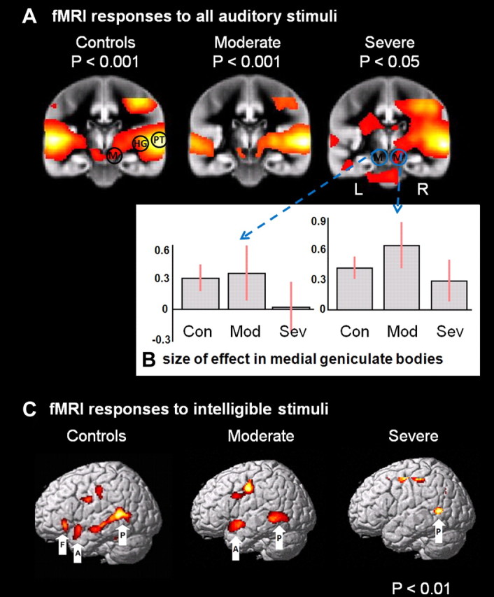
fMRI analysis, univariate analysis SPM{t} map. A, Coronal views (in the plane of the MGBs, y = −22) showing the SPM{t} map of the main contrast “all auditory”(speech and time-reversed speech > background scanner noise), for all three groups. Bilateral activations are seen in the MGBs and supratemporal plane for the controls and moderate group. There is less activity on the left for the severe group. Note that even at a very low threshold (p < 0.05 uncorrected), there is no activity in the severe group in left MGB. L, Left; R, right. The three regions are depicted on the right of the control group: M = MGB, HG, and PT, but were applied bilaterally to controls and moderates. For the severe group these three regions were used on the right, but only the PT could be used on the left. B, Effect sizes of BOLD response from left and right MGB. Con, Control; Mod, moderate; Sev, severe. C, The results of the intelligibility contrast for the three groups. The left panel shows activation for the normal subjects, the middle panel for moderate patients, and the rightmost panel for the severe patients. Labels: P, pSTS; A, aSTS; F, pOrb.
Table 4.
Functional imaging analysis, peak activations from the VOIs identified by the “all auditory” contrast across all three groups
| Coordinates |
Controls Z score | Moderate Z score | Severe Z score | |||
|---|---|---|---|---|---|---|
| x | y | z | ||||
| Supratemporal plane | ||||||
| 1. Left planum temporale | −66 | −22 | 8 | Inf† | 5.1‡ | 2.5 |
| Right planum temporale | 64 | −22 | 2 | Inf | 7.7 | 7.6 |
| 2. Left posteromedial Heschl's gyrus (A1) | −44 | −24 | 8 | Inf*,† | 3.2 | ns |
| Right posteromedial Heschl's gyrus (A1) | 46 | −24 | 6 | Inf | 6.6 | 6.0 |
| Medial geniculate nucleus | ||||||
| 3. Left | −22 | −22 | 0 | 3.3† | 2.2 | ns |
| Right | 22 | −22 | 0 | 5.3 | 4.2 | 2.4 |
Coordinates are in MNI space. The location and extent of these regions are illustrated in Figure 3, where numbers 1–4 relate to the key regions in the supratemporal plane. Asterisk (*), Controls > moderate patients at p < 0.001 uncorrected; dagger (†), controls > severe patients at p < 0.001 uncorrected for cortical structures or FWE corrected for small volume 8 mm radius for MGB; double dagger (‡), moderate patients > severe patients at p < 0.001.
Using standard SPMs, we found group differences in activation at three levels of the auditory hierarchy, but only in the left hemisphere. (1) Moderate patients had reduced activation compared to controls in left HG only, although this area was not significantly damaged in the moderate patients. (2) Severe patients had reduced activation relative to controls in all three levels of the left hemisphere hierarchy (MGB, HG and PT, although MGB was not significantly damaged in the severe patients). (3) Severe patients also had reduced activation compared to moderate patients in left PT only. The left MGB was not activated in the severe group, but this effect only reached significance when compared to the controls but not the moderate group. Reverse contrasts for these six regions and indeed any region in the supratemporal plane revealed no other significant differences.
To summarize the structural and functional differences between all three groups at each level of the auditory hierarchy on the left. (1) At the level of PT, the severely affected patients had significantly less gray matter than both the moderately affected patients and controls; this was mirrored by a reduced BOLD signal in this region relative to the other groups. (2) At the level of HG (anterolateral portion), the severe patients had significantly less gray matter than both the moderates and controls; however, both patient groups had a reduced BOLD signal here compared to the controls (extant, posteromedial portion). (3) At the level of the MGB there were no structural differences between the groups; however, the severely affected patients had significantly less BOLD signal here than the controls. Thus, as a rule, reduced activation was recorded at one level lower in the hierarchy than reduced structure.
DCM and BMA analysis of between-region responses to all-auditory stimuli
The aim of the DCM analyses was to test whether there were any differences between the three groups in terms of altered effective connectivity, i.e.: task-dependent, directed interactions between auditory regions. This can occur even when there are no group differences identified in the univariate analysis of the BOLD response (e.g., the three right hemisphere regions).
For the control subjects, the results of the estimated probability distributions for the 18 between-region connections are shown in the top row of Figure 4. Eleven connections had values significantly greater than zero; these are colored black in the figure. The only two nonsignificant interhemispheric connections were at the level of the MGBs, consistent with previous reports about the lack of a consistent interhemispheric connection at this level (Malobabić et al., 1990). We included connections between MGB and PT that bypass HG because of the evidence from macaque studies (Kaas and Hackett, 2000); however, these connections are sparse, and we only found evidence for one of these four connections being modulated by speech-like sounds. Likewise, the feedback connections between PT and HG were not significantly modulated in control subjects.
Figure 4.
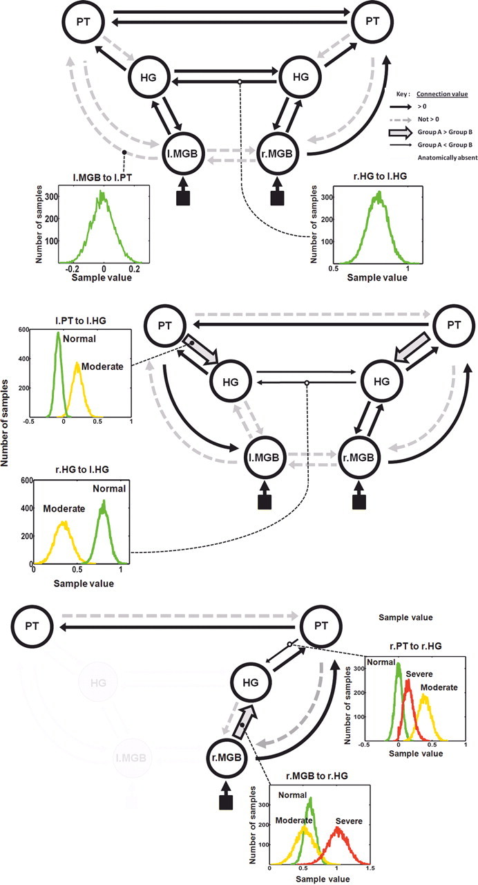
Bayesian Model Averaging result, multivariate analysis of data extracted from the VOIs. Connectivity results are shown for the three groups: top, controls; middle, moderate; and bottom, severe patient groups. The six VOIs are shown for the first two groups, only four of these could be used in the severe group; left HG and MGB were not activated in the SPM{t} analysis and appear as grayed out. Black arrows of standard thickness depict between-region connections significantly greater than zero; nonsignificant connection values are shown in gray dashed lines (see key top right). The circles around each region depict the within-region connections. Two connection distributions are shown in insets; these represent 10,000 samples across all subjects weighted by model probability (controls, green; moderates, amber; severe, red). For the moderate group two connections were significantly weaker than the controls (thin black arrows). Two connections were significantly stronger (thick arrows with gray inset). For the severe group one connection was significantly stronger than the moderates (thick arrow with gray inset), and one was significantly weaker (thin black arrow). l., Left; r., right.
Because the network model for the moderate group contained the same six regions, we were able to fit exactly the same DCMs as for the controls and compare the resulting distributions of connection strengths between these two groups on all 18 between-region connections. We found that 8 of the 18 between-region connections (black connections in middle row of Fig. 4) were significantly modulated by speech-like sounds. Two of these connections had significantly higher values than the control group (thick arrows with gray center), namely the feedback connections between PT and HG in both hemispheres, suggesting that moderate patients are more dependent on top-down processing (prediction signals) than normal subjects when listening to speech-like stimuli. Note that this finding of increased connectivity in moderately affected patients contrasts with the results of the conventional SPM analysis that did not identify any voxels with greater task-dependent activity in any of the six regions compared with the control subjects. In contrast, the two between-hemisphere connections at the level of the HGs were significantly weaker (thin arrows).
For the severe group we could only include four of the six regions in the DCMs (see Materials and Methods). Although left PT was significantly damaged, this structure is large enough for part of it to be significantly activated in this group (Tables 3 and 4, far right columns). Left HG activity was absent in the severe group, almost certainly because this region was more significantly damaged in the severe group compared with the moderate group (Table 3). More surprisingly, there was no significant activity in the left MGB, despite this region being structurally intact in all nine severe patients (Fig. 1B). We discuss potential explanations for this observation below. There was a significant activation of the remaining four regions (PT on the left and all three on the right), enabling us to generate a series of models using the same rules as for the normal subjects and moderate patient groups. Using BMA, we were then able to compare the connection strengths for all three groups across these shared eight between-region connections; the results are shown in the bottom row of Figure 4. We found that four of the eight connections were significantly modulated by speech-like sounds, with one of these connections having significantly higher vales than the moderate group (thick arrow with gray center): a feedforward connection from MGB to HG. In contrast, one connection was significantly weaker (thin arrow): a feedback connection from PT to HG.
Effects of intelligibility
The DCMs reported above describe an auditory network whose nodes were defined by contrasting all auditory speech-like stimuli (intelligible and time reversed) against no auditory stimulation. For completion, we also report the results from the SPM analysis of the differential contrast (intelligible vs time-reversed speech). These results have been reported for the control subjects elsewhere (Leff et al., 2008). In short, three areas in the dominant frontotemporal lobe were activated by intelligible speech: the anterior and posterior parts of the superior temporal sulcus (STS) and the pars orbitalis (POrb) of the inferior frontal gyrus; see Figure 3C. Intelligible speech increased activation in the pSTS (both patient groups, although only at trend significance in the severe patients) and in the aSTS (moderate patients only). POrb was not significantly activated in either patient group. Comparisons between the groups demonstrated significantly greater activity in the aSTS for controls > moderate patients > severe patients. The only other significant effect was in the pSTS with controls > severe patients (see Table 5). DCM analyses were not carried out on this contrast, as we only identified one region in the severe patient group.
Table 5.
Functional imaging analysis, peak activations from the VOIs identified by the “intelligibility” contrast across all three groups
| Coordinates |
Controls Z score | Moderate Z score | Severe Z score | |||
|---|---|---|---|---|---|---|
| x | y | z | ||||
| Left hemisphere | ||||||
| 1. Pars orbitalis (F) | −46 | 28 | −6 | 2.73 | ns | ns |
| 2. Anterior STS (A) | −56 | 10 | −12 | 3.44† | 2.69 | ns |
| 3. Posterior STS (P) | −54 | −46 | 12 | 3.78† | 3.85‡ | 2.59 |
Coordinates are in MNI space and represent an average across the three groups. The location and extent of these regions are illustrated in Figure 3C, where letters F is frontal, A is aSTS, and P is pSTS. Bold results are p < 0.05 FWE corrected for small volume 8 mm radius for the region; italicized Z score, p < 0.1; and ns Z score, p > 0.1. Dagger (†), Controls > severe patients; double dagger (‡), moderate patients > severe patients.
Discussion
The patients taking part in this study were selected on the basis of their impaired performance on tests of speech comprehension. The first unexpected finding was that the distribution of comprehension scores varied in a strongly bimodal manner (Fig. 1A); however, tests on a much larger group of aphasic patients from which they were drawn confirmed this pattern. The moderate group had normal single word comprehension but impaired sentence level comprehension, while the severe group was impaired at the single word level and significantly worse at sentences. We investigated differences in brain structure and function that might explain this.
As expected, both patient groups had significant damage to gray matter in the left supratemporal plane. There was common damage to the anterior portion of the planum polare, the posterior insula, the caudate, and the putamen, and to white matter in temporal, parietal, and frontal portions of the arcuate fasciculus. It is likely that damage to these gray and white matter structures caused the substantial impairments in object naming and verbal fluency that were seen to exist with the same severity in both groups, along with the observed mild impairment in auditory word discrimination [Psycholinguistic Assessment of Language Processing in Aphasia (PALPA)] scores. It should be noted however, that segmentation of the patients' images is likely to be imperfect due to the presence of the stroke damage. As such, inferences are best based on a coarse, rather than fine-grained, spatial scale.
We then looked for structural differences that might explain the behavioral differences between the two patient groups. There was no significant difference in terms of total lesion volume. Compared to the moderate patients, the severe group had sustained significantly more damage to three left hemisphere gray matter regions: the posterior insula and two supratemporal regions of auditory cortex, HG and PT. The severe group had also sustained significantly more damage to the white matter underlying the superior temporal lobe and the temporal and parietal parts of the arcuate fasciculus. This pattern of damage is likely to have caused their significant impairment of spoken single word and sentence level comprehension.
We then proceeded to investigate the effect of this damage upon the functional architecture of the auditory system using an fMRI contrast to identify activation in lower-level regions of the auditory system. In the moderate patients all six of these regions were structurally intact; the effects of the damage to multimodal regions higher in the auditory hierarchy were apparent in the activity and/or connectivity of these lower regions, particularly for left HG. The significantly reduced activity in this region can be seen in the standard SPM{t} maps (Table 3). Additionally, the DCM analysis revealed that the two between-hemisphere connections at this level were reduced in strength compared to normal subjects; also, no significant connections were identified linking left MGB to HG. These two findings suggest that, in moderate patients, broadband auditory stimuli influence the left hemisphere only after being filtered by the right hemisphere, with the main conduit at the level of the PTs. Two connections had significantly higher values; these are both feedback or top-down connections (from PT to HG). Interpreted within the predictive coding framework (Rao and Ballard, 1999; Friston, 2005), this represent a stronger influence of predictions, suggesting that moderate patients rely more on abstracted sensory memories than controls when processing speech-like sounds.
The patients in the severe group had considerably more damage to their dominant supratemporal plane compared to both normal controls and the moderate patients, with damage to both lower (predominantly unimodal) and higher (multimodal) areas in the left hemisphere (Fig. 2, Table 3). In particular, compared to the moderate patients, they had significantly less gray matter in HG and PT, with additional damage to the white matter underlying these structures, the middle longitudinal fasciculus (Schmahmann and Pandya, 2006). The effect of this on the standard SPM{t} maps was very interesting. Unsurprisingly, the severe group had no significant BOLD activity in left HG. They did, however, have some in PT, although significantly less than the moderate group (Table 3). This structure is relatively large and thus was not completely damaged in any of the severe patients (Westbury et al., 1999). The most surprising result was the lack of any task-dependent BOLD response in left MGB, despite this region being structurally intact in all subjects. The explanation for this is unlikely to be due to a simple, nonspecific effect of stroke, as the moderate patients had a higher mean BOLD response in both MGBs compared with the controls, and the severe patients had a mean response similar to the controls on the right (Fig. 3B). All patients had an intact MGB on the left and no evidence of a hearing deficit other than would be expected for their age on pure tone audiometry. The stimuli were presented binaurally, so it is reasonable to assume that there was no imbalance in the bottom-up auditory inputs. The only significant anatomical differences between the two patient groups in the supratemporal plane was damage to HG, PT, and the white matter deep to these structures, both of which have direct synaptic connections with MGB (Kaas and Hackett, 2000). Given that task-dependent BOLD responses reflect synaptic activity (neuronal inputs) more than spiking activity (neuronal outputs) (Viswanathan and Freeman, 2007), a plausible explanation for this lack of a response is the loss of feedback connections, primarily from HG to MGB, a form of deafferentation from above. As it is probable that neurons in the MGB are receiving and reacting to ascending auditory input, the lack of activation observed is consistent with the normal task-dependent BOLD response in the MGB being predominantly driven by modulatory influence from the cortex.
We were only able to compare connection strength values between the three groups over common connections. The severe group was missing two of the six regions that were part of the network modeled for controls and moderate patients. They were performing the same task as the other two groups, but with reduced neural machinery. In terms of feedforward connections, compared with controls, they had one significantly increased connection, from right MGB to right HG. In terms of feedback connections, one was significantly reduced: right PT to right HG. The predictive coding account (Rao and Ballard, 1999) suggests that one of the consequences of stroke in severely affected patients is a reduced role of top-down influences on early auditory areas. These less veridical predictions about speech-like sounds appear to originate in the right hemisphere.
These data are cross-sectional; nevertheless, given that the moderate group showed increased connectivity of backward connections while the severe group had reduced connectivity for some of the same connections, it is reasonable to postulate that these differences in effective connectivity in both hemispheres may be supporting residual function in the moderate group. Longitudinal data would be required to definitively prove this, e.g., the effect of repetitive transcranial magnetic stimulation (rTMS) therapy in stoke patients with hand weakness (Grefkes et al., 2010).
The moderate group had damage to multimodal left hemisphere auditory areas and it may well be, as is commonly assumed, that their aphasic disorder was a direct result of this. However, it is interesting to note two things. First, this damage had repercussions on structurally intact areas lower down in the auditory hierarchy: the functional interactions of unimodal auditory areas were altered in both patient groups. Second, the severe group did not have significantly more damage than the moderate group to multimodal cortex; rather, they had additional damage to dominant unimodal auditory cortex. This suggests that patients with aphasia may have damage affecting the function of “early” auditory areas critically contributing to their impairments. This is supported by evidence that aphasic patients are impaired on tasks using complex, nonspeech auditory stimuli (Saygin et al., 2003).
The debate over whether recovery from aphasia is mainly a property of the left or right hemisphere dates back to the 19th century (Gowers, 1887), as does the influence of the right hemisphere in aphasia, i.e., whether it supports residual performance or causes residual impairment (Moscovitch, 1976). The advent of functional imaging has served to intensify this debate with considerable evidence to support both sides of the argument (Heiss et al., 2003; Price and Crinion, 2005; Crosson et al., 2007). Our results also provide evidence for both sides. The intelligibility contrast suggests that the left hemisphere remains important for processing lexical aspects of speech, regardless of aphasia severity; while the connectivity analysis stresses the importance of the right hemisphere, as evidenced by the main input into the auditory system being via right MGB in the severe group and the asymmetry (right to left) at the PT level in both patient groups. We propose that both hemispheres have a role in supporting recovery, particularly when speech perception is affected. For patients with persistent, moderate auditory perceptual deficits, the interhemispheric connections between HGs appear to be weaker than normal; however, symmetrical modulation of top-down connections may compensate for this. For patients with persistent, severe auditory perceptual deficits, these top-down effects are significantly reduced in the unaffected hemisphere. Given this, it is possible that the beneficial effects of language therapy may be expressed at the network level of connectivity of the remaining auditory system, rather than in any given region, be it in the left or right hemisphere.
Footnotes
This work was supported by The Wellcome Trust, the James S. MacDonnell Foundation (conducted as part of the Brain Network Recovery Group initiative), the NIHR CBRC at University College Hospitals, and the University Research Priority Program “Foundations of Social Human Behaviour” at the University of Zurich.
This paper is dedicated to the memory of our dear friend and colleague, neuroscientist Dr Thomas Schofield, who worked with the aphasic patients taking part in this study for five years. Tom tragically lost his life in a road-traffic accident.
References
- Abutalebi J, Rosa PA, Tettamanti M, Green DW, Cappa SF. Bilingual aphasia and language control: a follow-up fMRI and intrinsic connectivity study. Brain Lang. 2009;109:141–156. doi: 10.1016/j.bandl.2009.03.003. [DOI] [PubMed] [Google Scholar]
- Ashburner J, Friston KJ. Voxel-based morphometry—the methods. Neuroimage. 2000;11:805–821. doi: 10.1006/nimg.2000.0582. [DOI] [PubMed] [Google Scholar]
- Ashburner J, Friston KJ. Unified segmentation. Neuroimage. 2005;26:839–851. doi: 10.1016/j.neuroimage.2005.02.018. [DOI] [PubMed] [Google Scholar]
- Boersma P. Praat, a system for doing phonetics by computer. Glot Int. 2001;5:341–345. [Google Scholar]
- Brodersen KH, Schofield TM, Leff AP, Ong CS, Lomakina EI, Buhmann JM, Stephan KE. Generative embedding for model-based classification of FMRI data. PLoS Comput Biol. 2011;7:e1002079. doi: 10.1371/journal.pcbi.1002079. [DOI] [PMC free article] [PubMed] [Google Scholar]
- Crinion J, Price CJ. Right anterior superior temporal activation predicts auditory sentence comprehension following aphasic stroke. Brain. 2005;128:2858–2871. doi: 10.1093/brain/awh659. [DOI] [PubMed] [Google Scholar]
- Crosson B, McGregor K, Gopinath KS, Conway TW, Benjamin M, Chang YL, Moore AB, Raymer AM, Briggs RW, Sherod MG, Wierenga CE, White KD. Functional MRI of language in aphasia: a review of the literature and the methodological challenges. Neuropsychol Rev. 2007;17:157–177. doi: 10.1007/s11065-007-9024-z. [DOI] [PMC free article] [PubMed] [Google Scholar]
- Deichmann R, Schwarzbauer C, Turner R. Optimisation of the 3D MDEFT sequence for anatomical brain imaging: technical implications at 1.5 and 3 T. Neuroimage. 2004;21:757–767. doi: 10.1016/j.neuroimage.2003.09.062. [DOI] [PubMed] [Google Scholar]
- Friston K. A theory of cortical responses. Philos Trans R Soc Lond B Biol Sci. 2005;360:815–836. doi: 10.1098/rstb.2005.1622. [DOI] [PMC free article] [PubMed] [Google Scholar]
- Friston KJ, Holmes AP, Worsley KJ, Poline JB, Frith CD, Frackowiak RSJ. Statistical parametric maps in functional imaging: a general linear approach. Human Brain Mapp. 1995;2:189–210. [Google Scholar]
- Friston KJ, Penny W, Phillips C, Kiebel S, Hinton G, Ashburner J. Classical and Bayesian inference in neuroimaging: theory. Neuroimage. 2002a;16:465–483. doi: 10.1006/nimg.2002.1090. [DOI] [PubMed] [Google Scholar]
- Friston KJ, Glaser DE, Henson RN, Kiebel S, Phillips C, Ashburner J. Classical and Bayesian inference in neuroimaging: applications. Neuroimage. 2002b;16:484–512. doi: 10.1006/nimg.2002.1091. [DOI] [PubMed] [Google Scholar]
- Friston KJ, Harrison L, Penny W. Dynamic causal modelling. Neuroimage. 2003;19:1273–1302. doi: 10.1016/s1053-8119(03)00202-7. [DOI] [PubMed] [Google Scholar]
- Friston K, Mattout J, Trujillo-Barreto N, Ashburner J, Penny W. Variational free energy and the Laplace approximation. Neuroimage. 2007;34:220–234. doi: 10.1016/j.neuroimage.2006.08.035. [DOI] [PubMed] [Google Scholar]
- Gowers WR. Lectures on the diagnosis of diseases of the brain. London: Churchill; 1887. [Google Scholar]
- Grefkes C, Nowak DA, Wang LE, Dafotakis M, Eickhoff SB, Fink GR. Modulating cortical connectivity in stroke patients by rTMS assessed with fMRI and dynamic causal modeling. Neuroimage. 2010;50:233–242. doi: 10.1016/j.neuroimage.2009.12.029. [DOI] [PMC free article] [PubMed] [Google Scholar]
- Heiss WD, Thiel A, Kessler J, Herholz K. Disturbance and recovery of language function: correlates in PET activation studies. Neuroimage. 2003;20(Suppl 1):S42–S49. doi: 10.1016/j.neuroimage.2003.09.005. [DOI] [PubMed] [Google Scholar]
- Hickok G, Okada K, Barr W, Pa J, Rogalsky C, Donnelly K, Barde L, Grant A. Bilateral capacity for speech sound processing in auditory comprehension: evidence from Wada procedures. Brain Lang. 2008;107:179–184. doi: 10.1016/j.bandl.2008.09.006. [DOI] [PMC free article] [PubMed] [Google Scholar]
- Kaas JH, Hackett TA. Subdivisions of auditory cortex and processing streams in primates. Proc Natl Acad Sci U S A. 2000;97:11793–11799. doi: 10.1073/pnas.97.22.11793. [DOI] [PMC free article] [PubMed] [Google Scholar]
- Landgrebe M, Langguth B, Rosengarth K, Braun S, Koch A, Kleinjung T, May A, de Ridder D, Hajak G. Structural brain changes in tinnitus: grey matter decrease in auditory and non-auditory brain areas. Neuroimage. 2009;46:213–218. doi: 10.1016/j.neuroimage.2009.01.069. [DOI] [PubMed] [Google Scholar]
- Leff AP, Schofield TM, Stephan KE, Crinion JT, Friston KJ, Price CJ. The cortical dynamics of intelligible speech. J Neurosci. 2008;28:13209–13215. doi: 10.1523/JNEUROSCI.2903-08.2008. [DOI] [PMC free article] [PubMed] [Google Scholar]
- Malobabić S, Puskas L, Vujasković G. Golgi morphology of the neurons in frontal sections of human interthalamic adhesion. Acta Anat. 1990;139:234–238. [PubMed] [Google Scholar]
- Meinzer M, Harnish S, Conway T, Crosson B. Recent developments in functional and structural imaging of aphasia recovery after stroke. Aphasiology. 2011;25:271–290. doi: 10.1080/02687038.2010.530672. [DOI] [PMC free article] [PubMed] [Google Scholar]
- Moscovitch M. On the representation of language in the right hemisphere of right-handed people. Brain Lang. 1976;3:47–71. doi: 10.1016/0093-934x(76)90006-7. [DOI] [PubMed] [Google Scholar]
- Noppeney U, Penny WD, Price CJ, Flandin G, Friston KJ. Identification of degenerate neuronal systems based on intersubject variability. Neuroimage. 2006;30:885–890. doi: 10.1016/j.neuroimage.2005.10.010. [DOI] [PubMed] [Google Scholar]
- Pandya DN. Anatomy of the auditory cortex. Rev Neurol. 1995;151:486–494. [PubMed] [Google Scholar]
- Penhune VB, Zatorre RJ, MacDonald JD, Evans AC. Interhemispheric anatomical differences in human primary auditory cortex: probabilistic mapping and volume measurement from magnetic resonance scans. Cereb Cortex. 1996;6:661–672. doi: 10.1093/cercor/6.5.661. [DOI] [PubMed] [Google Scholar]
- Penny WD, Stephan KE, Daunizeau J, Rosa MJ, Friston KJ, Schofield TM, Leff AP. Comparing families of dynamic causal models. PLoS Comput Biol. 2010;6:e1000709. doi: 10.1371/journal.pcbi.1000709. [DOI] [PMC free article] [PubMed] [Google Scholar]
- Price CJ, Crinion J. The latest on functional imaging studies of aphasic stroke. Curr Opin Neurol. 2005;18:429–434. doi: 10.1097/01.wco.0000168081.76859.c1. [DOI] [PubMed] [Google Scholar]
- Price CJ, Seghier ML, Leff AP. Predicting language outcome and recovery after stroke: the PLORAS system. Nat Rev Neurol. 2010;6:202–210. doi: 10.1038/nrneurol.2010.15. [DOI] [PMC free article] [PubMed] [Google Scholar]
- Rao RP, Ballard DH. Predictive coding in the visual cortex: a functional interpretation of some extra-classical receptive-field effects. Nat Neurosci. 1999;2:79–87. doi: 10.1038/4580. [DOI] [PubMed] [Google Scholar]
- Saur D, Lange R, Baumgaertner A, Schraknepper V, Willmes K, Rijntjes M, Weiller C. Dynamics of language reorganization after stroke. Brain. 2006;129:1371–1384. doi: 10.1093/brain/awl090. [DOI] [PubMed] [Google Scholar]
- Saygin AP, Dick F, Wilson SM, Dronkers NF, Bates E. Neural resources for processing language and environmental sounds: evidence from aphasia. Brain. 2003;126:928–945. doi: 10.1093/brain/awg082. [DOI] [PubMed] [Google Scholar]
- Schmahmann JD, Pandya DN. Fibre pathways of the brain. New York: Oxford UP; 2006. [Google Scholar]
- Seghier ML, Ramlackhansingh A, Crinion J, Leff AP, Price CJ. Lesion identification using unified segmentation-normalisation models and fuzzy clustering. Neuroimage. 2008;41:1253–1266. doi: 10.1016/j.neuroimage.2008.03.028. [DOI] [PMC free article] [PubMed] [Google Scholar]
- Stephan KE, Harrison LM, Kiebel SJ, David O, Penny WD, Friston KJ. Dynamic causal models of neural system dynamics:current state and future extensions. J Biosci. 2007;32:129–144. doi: 10.1007/s12038-007-0012-5. [DOI] [PMC free article] [PubMed] [Google Scholar]
- Stephan KE, Penny WD, Moran RJ, den Ouden HE, Daunizeau J, Friston KJ. Ten simple rules for dynamic causal modeling. Neuroimage. 2010;49:3099–3109. doi: 10.1016/j.neuroimage.2009.11.015. [DOI] [PMC free article] [PubMed] [Google Scholar]
- Swinburn K, Porter G, Howard D. Comprehensive aphasia test. New York: Psychology Press; 2004. [Google Scholar]
- Viswanathan A, Freeman RD. Neurometabolic coupling in cerebral cortex reflects synaptic more than spiking activity. Nat Neurosci. 2007;10:1308–1312. doi: 10.1038/nn1977. [DOI] [PubMed] [Google Scholar]
- Westbury CF, Zatorre RJ, Evans AC. Quantifying variability in the planum temporale: a probability map. Cereb Cortex. 1999;9:392–405. doi: 10.1093/cercor/9.4.392. [DOI] [PubMed] [Google Scholar]