A filtered backprojection MAP algorithm with nonuniform sampling and noise modeling

Abstract

Purpose: The goal of this paper is to extend our recently developed FBP (filtered backprojection) algorithm, which has the same characteristics of an iterative Landweber algorithm, to an FBP algorithm with the same characteristics of an iterative MAP (maximum a posteriori) algorithm. The newly developed FBP algorithm also works when the angular sampling interval is not uniform. The projection noise variance can be modeled using a view-based weighting scheme.

Methods: The new objective function contains projection noise model dependent weighting factors and image dependent prior (i.e., a Bayesian term). The noise weighting is view-by-view based. For the first time, the FBP algorithm is able to model the projection noise. Based on the formulation of the iterative Landweber MAP algorithm, a frequency-domain window function is derived for each iteration of the Landweber MAP algorithm. As a result, the ramp filter and the windowing function are both modified by the Bayesian component. This new FBP algorithm can be applied to a projection data set that is not uniformly sampled.

Results: Computer simulations show that the new FBP-MAP algorithm with window function index k and the iterative Landweber MAP algorithm with iteration number k give similar reconstructions in terms of resolution and noise texture. An example of transmission x-ray CT shows that the noise modeling method is able to significantly reduce the streaking artifacts associated with low-dose CT.

Conclusions: View-based noise weighting scheme can be introduced to the FBP algorithm as a weighting factor in the window function. The new FBP algorithm is able to provide similar results to the iterative MAP algorithm if the ramp filter is modified with a additive term. Nonuniform sampling and sensitivity can be accommodated by proper backprojection weighting.

INTRODUCTION

The filtered backprojection (FBP) algorithm is simple and fast, and can be used to reconstruct images in nuclear medicine, x-ray CT, or even MRI for some special data acquisition methods.¹ Compared with iterative reconstruction algorithms, the FBP algorithm generally produces noisier images, even when the iterative algorithm (e.g., the iterative Landweber algorithm) does not model the projection noise or does not model the projection noise correctly.^{2, 3} As a result, the FBP algorithm has gradually been replaced by iterative image reconstruction algorithms. Recently, we have developed a windowed FBP algorithm that is able to produce similar images to those reconstructed by the iterative Landweber algorithm.⁴ One goal of this paper is to modify this windowed FBP algorithm so that it can produce similar images to those reconstructed by the iterative Landweber MAP algorithm. Another goal of this paper is to extend the windowed FBP algorithm to model the projection data noise.

Iterative maximum a posteriori (MAP) algorithms can produce noise/resolution balanced images and have wide applications.^{5, 6, 7, 8} Due to their huge projection operator matrix size, MAP algorithms use iterative methods to optimize the objective function. Recently, Cao et al. proposed a special representation of the huge sparse projection matrix so that the condensed projection matrix can be stored in a computer and a noniterative reconstruction becomes possible.⁹ However, this sparse-matrix transformation approach is not easy to implement. Three new methods of the FBP algorithms are presented in Sec. 2. The new methods are practical and can include some noise information and image prior information in the FBP reconstruction.

METHODS

A simple FBP-MAP approach is derived in Sec. 2A; the implementation of this FBP-MAP algorithm is almost the same as a regular FBP algorithm. Nonuniform angular sampling is considered in Sec. 2B. In Sec. 2C, computer implementation issues are considered. In Sec. 2D, the noise modeling strategy is introduced, and a noise variance weighted FBP algorithm is derived.

A new FBP algorithm that emulates an iterative MAP algorithm

A typical MAP (maximum a posteriori) algorithm is to optimize the Bayesian estimation as

$$\hat{X}=\arg \underset{X}{\min }\{{\Vert P-\mathit{AX}\Vert }^2+\beta X^T\mathit{RX}\}.$$ (1)

In the context of tomography, A in Eq. 1 is the projection matrix, X is the image array written as a column vector, P is the projection array written as a column vector, and β is a relative weighting factor that adjusts the importance of the Bayesian term X^TRX relative to the fidelity term ||P-AX||². The square matrix R in Eq. 1 can be understood in such a way that X is modeled by a Gaussian random field with a covariance matrix R⁻¹. In practice, X is not random, the matrix R is used to enforce some smoothness of the image so that the reconstruction is not too sensitive to noise. One way to promote the smoothness is to suppress the difference between the central pixel value and its neighbors. A Laplace operator that is the second-order derivative, for example, can be used in the matrix R.

The optimization problem 1 has a quadratic objective function, so the solution can be obtained by the Landweber algorithm

$$X^{(k+1)}=X^{(k)}+\alpha [A^T(P-{\mathit{AX}}^{(k)})-\beta {\mathit{RX}}^{(k)}],$$ (2)

where A^T is the backprojection matrix, X^(k) is the estimated image at the kth iteration, and α > 0 is the step-size. This recursive relation can be rewritten as a nonrecursive expression as

$$\begin{array}{c}{X}^{(k+1)}=X^{(k)}+\alpha [A^T(P-{\mathit{AX}}^{(k)})-\beta {\mathit{RX}}^{(k)}]=\alpha A^{T}P+(I-\alpha A^{T}A-\alpha \beta R)X^{(k)}=[\sum _{n=0}^k{(I-\alpha A^{T}A-\alpha R)}^n]\alpha A^{T}P\end{array}+{(I-\alpha A^{T}A-\alpha R)}^{k+1}{X}^{(0)}.$$ (3)

If the initial image X⁽⁰⁾ is set to zero, the result from k iterations of the Landweber algorithm is

$$X^{(k)}=\alpha \left[\sum _{n=0}^{k-1}{(I-\alpha A^{T}A-\alpha \beta R)}^n\right]A^{T}P.$$ (4)

This noniterative expression of the Landweber algorithm resembles a “backproject first, then filter” algorithm, in the sense that the projection data P are first backprojected by the operator A^T and then filtered by $\alpha [{\sum }_{n=0}^{k-1}{(I-\alpha A^{T}A-\alpha \beta R)}^n]$. When the positive real number (i.e., step-size) α is small enough, the Landweber algorithm will converge and we have

$$\begin{array}{c}\alpha \left[\sum _{n=0}^{k-1}{(I-\alpha A^{T}A-\alpha \beta R)}^n\right]\to {(A^{T}A+\beta R)}^{-1}\mathrm{as}k\to \infty ,\end{array}$$ (5)

if ${(A^{T}A+\beta R)}^{-1}$ exists, otherwise ${(A^{T}A+\beta R)}^{-1}$ is replaced by a generalized inverse. For a finite k, we have

$$\begin{array}{c}\alpha \left[\sum _{n=0}^{k-1}{(I-\alpha A^{T}A-\alpha \beta R)}^n\right]={(A^{T}A+\beta R)}^{-1}\times [I-{(I-\alpha A^{T}A-\alpha \beta R)}^k].\end{array}$$ (6)

The proofs of the above equations are available in a review paper by Schafer et al.¹⁰

The Landweber algorithm is a linear algorithm, but it may not be shift-invariant. The PSF (point spread function) of the combined operator of projection-and-backprojection plus the Bayesian term R, A^TA + βR, is almost shift-invariant in the central region of the image array, which can be verified by putting a point source in the image, and then performing the projection-backprojection operation. After the operation, the resultant blurred point source image is almost shift-invariant if the point source is close to the center of the image array. When the point source is close to the array edges, the blurred point source image is no longer shift-invariant. If we use a large image array (say, the array size is twice as large as the image object) in the iterative Landweber MAP algorithm, the PSF can be considered shift-invariant in the object region.

As shown in image reconstruction textbooks and in our previous paper, if the projection operator A is the line-integral (i.e., the Radon transform) in the two-dimensional (2D) space and A^T is the adjoint operator (i.e., the backprojection transform), the combined operator of projection-and-backprojection, A^TA, is the 2D convolution of the original image with a 2D kernel 1/r, where $r=\sqrt{x^2+y^2}$ in the x-y Cartesian coordinates.¹¹ The 2D ramp filter is able to cancel the 1/r blurring effect.¹⁰ In this ideal situation, the (A^TA) operation is a 1/r convolution, the (A^TA)⁻¹ operation is 2D ramp filtering, and $[I-{(I-\alpha A^{T}A-\alpha \beta R)}^k]$ in Eq. 6 can be treated as a window function in the frequency-domain

$$W_k({\nu }_x,{\nu }_y)=1-{(1-\alpha (1/\Vert \stackrel{\rightharpoonup }{\nu }\Vert +\beta h(\Vert \stackrel{\rightharpoonup }{\nu }\Vert )))}^k,\hspace{1em}\mathrm{with}\hspace{1em}\Vert \stackrel{\rightharpoonup }{\nu }\Vert =\sqrt{{\nu }_x^2+{\nu }_y^2},$$ (7)

where ν_x and ν_y are the frequencies with respect to x and y, respectively, $\stackrel{\rightharpoonup }{\nu }=(v_x,v_y)$ is the 2D frequency vector, and h is the Fourier transform of R when R is expressed as a convolution kernel. Thus, the conceptual shift-invariant Landweber algorithm is equivalent to: first, backprojecting the data into the image domain; second, filtering the backprojected image with a 2D windowed ramp filter defined in Eq. 7.

Nonuniform angular sampling

The conventional FBP algorithm assumes that the object is uniformly sampled. However, one can use variable sampling strategies, such as sampling the more important angular range with a smaller angular interval and sampling the less important angular range with a larger angular interval. The angular sampling can be normalized in the backprojection as a weighting function. The backprojection is an integral over the sampling angle. Angular sampling density compensation can be achieved by using a normalization factor in the backprojection integral, which is essentially a Jacobian factor. Mathematically, a backprojection image can be expressed as

$$b(x,y)={\int }_0^{\pi }{p(t,\theta )|}_{t=x\cos \theta +y\sin \theta }d\theta ,$$ (8)

where p can be the raw projections at angle θ if the algorithm requires the raw projections be backprojected first, p can also be the filtered projections at angle θ if an FBP algorithm is used, and t indicates the detector bin location. A simple discrete implementation of Eq. 8 is given as

$$b(i,j)={\frac{\pi }{M}\sum _{m=1}^{M}p(n,m)|}_{n=\mathit{INT}[x\cos \theta +y\sin \theta ]},$$ (9)

where n is the detector location index, m is the projection angle index, M is the total number of views at which projections are acquired, and “INT” is used to indicate the nearest neighbor interpolation. In fact, a typical implementation does not use an “INT” function, but uses linear interpolation between two neighboring detector bins. For the purposes of illustration, we stay with the simple implementation (9). When the angular sampling is not uniform, it obeys a density function d(θ), which is the number of views per unit angle. For example, if the sampling interval is 1° for $0\le \theta <\pi /4$ and 3° for $\pi /4\le \theta <\pi$, then the density function is

$$d(\theta )=\{\begin{array}{c}1\hspace{1em}\mathrm{for}\hspace{1em}0\le \theta <\pi /4\\ 1/3\hspace{1em}\mathrm{for}\hspace{1em}\pi /4\le \theta <\pi ,\end{array}$$ (10)

and the backprojection 9 can be modified as

$$\begin{array}{c}b(i,j)=\left(\pi /\sum _{m=1}^M\frac{d(1)}{d(m)}\right)\sum _{m=1}^M\frac{d(1)}{d(m)}{p(n,m)|}_{n=\mathrm{INT}[x\cos \theta +y\sin \theta ]}.\end{array}$$ (11)

Here, the sampling density function is a function of the angle index m, instead of the actual angle θ.

Implementation

In fact, a “backproject first, then filter” algorithm is equivalent to an FBP algorithm, which filters the projections first, then backprojects.^{4, 11} The one-dimensional (1D) frequency-domain filter in the FBP algorithm is the 1D profile of the 2D filter in the “backproject first, then filter” algorithm.^{4, 11} Therefore, an iterative-Landweber-MAP-equivalent FBP-MAP algorithm can be obtained, and the implementation steps are

Step 1: Perform the 1D Fourier transform of the projection at each view.

Step 2: Filter the frequency-domain data with a 1D windowed ramp filter

$$\begin{array}{c}{H}_k({\nu }_t)=[1-{(1-\alpha (1/\left|{\nu }_t\right|+\beta h(\left|{\nu }_t\right|)))}^k]/|1/\left|{\nu }_t\right|+\beta h(\left|{\nu }_t\right|)|\hspace{1em}\mathrm{and}\hspace{1em}{H}_k(0)=0,\end{array}$$ (12)

where ν_t is the frequency with respect to the linear variable on the 1D detector.

Step 3: Perform a 1D inverse Fourier transform of the filtered data.

Step 4: Perform the backprojection.

When k = ∞ and β = 0, 12 is the ramp filter in the conventional FBP algorithm.

An alternative way to implement this new FBP algorithm is to use convolution to replace the Fourier-domain projection data filtering. The convolution kernel is the inverse Fourier transform of the Fourier-domain filter function H_k(v_t) defined in Eq. 12.

Similarly, two ways can be used to implement the proposed FBP algorithm in the form of “first backprojection, then filtering.” The filtering can be performed in the Fourier-domain as multiplication, or can be performed in the spatial domain as convolution.

Noise variance weighted FBP algorithm

In order to make the derivation more clearly, we turn off the Bayesian term in the objective function by setting β = 0. When noise is modeled, Eq. 1 becomes

$$\hat{X}=\arg \underset{X}{\min }\{{\Vert P-\mathit{AX}\Vert }_W^2\}=\arg \underset{X}{\min }\{{(P-\mathit{AX})}^{T}W(P-\mathit{AX})\},$$ (13)

w?>where W is a diagonal square matrix with weighting factors as the diagonal elements. In principle, a larger weighting factor is assigned to a less noisy measurement and a smaller factor for a noisier measurement. For example, the weighting factors can be chosen as a function of the noise variance of the corresponding projection. Since an FBP algorithm has a shift-invariance PRF, we require that the weighting factor has the same value for all projections in each view. In x-ray CT imaging, this weighting factor assignment strategy is reasonable. When the x-rays travel in the direction from shoulder to shoulder, the projections are noisier than when the x-rays travel in the direction from the front to the back of the torso. If an iterative Landweber algorithm is used to solve 13, following the similar derivation as in Sec. 2A and replacing A^TA by A^TWA everywhere, the result of the kth iteration is given as

$$X^{(k)}=\alpha \left[\sum _{n=0}^{k-1}{(I-\alpha A^T\mathit{WA})}^n\right]A^T\mathit{WP}=[I-{(I-\alpha A^T\mathit{WA})}^k]{(A^T\mathit{WA})}^{-1}{A}^T\mathit{WP}.$$ (14)

In this symbolic derivation, we assume that ${(A^T\mathit{WA})}^{-1}=A^{-1}{W}^{-1}{(A^T)}^{-1}$ exists. Thus, Eq. 14 is simplified as

$$X^{(k)}=[I-{(I-\alpha A^T\mathit{WA})}^k]A^{-1}P.$$ (15)

Following the same steps as in Sec. 2C, Eq. 15 can be turned into an FBP algorithm and the windowed ramp filter is given as

$$H_k({\nu }_t)=[1-{(1-\alpha (w_{\mathrm{view}}/\left|{\nu }_t\right|))}^k]·\left|{\nu }_t\right|\hspace{1em}\mathrm{and}\hspace{1em}{H}_k(0)=0,$$ (16)

where w_view is the weighting factor for the projection at a particular view. The implementation procedure of this noise variance weighted FBP algorithm is the same to that discussed in Sec. 2C except that 12 is replaced by Eq. 16.

COMPUTER SIMULATION RESULTS

FBP-MAP

Some computer simulations are provided in this section. The Shepp-Logan phantom¹ was used in computer simulation studies. A 1D parallel-hole detector was rotated over 180° with 120 views and 128 detector bins on the detector. The images were reconstructed in a 256 × 256 array and the central 128 × 128 array was used for display and image comparison studies. Noiseless data were used for resolution comparison studies. Poisson noise was added to the projection data in noise studies, where 100 noise realizations were used to generate the signal-to-noise (S/N) images. The signal-to-noise ratio is defined as the mean value over the standard deviation. Ensemble mean and ensemble standard deviation were calculated for each image pixel with 100 noise realizations.

In all computer simulations, both the iterative MAP algorithm and the new FBP-MAP algorithm used the same step-size α = 0.5, the same parameter β (=  0.1 and 0.3) and the same iteration indices k = 2, 20, and 200, respectively. The requirement of choosing parameter α is that $\alpha /\left|{\nu }_t\right|\le 1$ in the newly developed FBP-MAP algorithm and $\alpha w_{\mathrm{view}}/\left|{\nu }_t\right|\le 1$ in the newly developed noise variance weighted FBP algorithm, where w_view is a noise weighting factor. In order to use the same parameter α = 0.5, we scaled the iterative algorithm’s projection/backprojection operator A^TA by 0.00005, that is

$$\begin{array}{c}{X}^{(k+1)}=X^{(k)}+\alpha [0.00005·A^T(P-{\mathit{AX}}^{(k)})-\beta {\mathit{RX}}^{(k)}].\end{array}$$ (17)

This value of 0.00005 and the parameter α were selected by trial-and-error. If the step-size α was chosen to be too large, the iterative algorithm would diverge and the FBP algorithm would produce unreasonable images. In Eq. 13, RX^(k) was implemented as a two-dimensional convolution with a convolution kernel as shown in Fig. 1.

Figure 1.

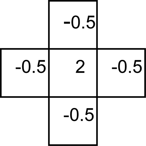
The 2D convolution kernel used in the iterative MAP algorithm to promote the smoothness of the image.

In the FBP-MAP algorithm, the Bayesian operator R was a Laplacian, whose convolution kernel is {−0.5, 1, −0.5}. The discrete Fourier transform of this kernel is h(n), which is a constant 1 minus a cosine function

$$h(n)=1-\cos \left(n\frac{2\pi }{N}\right),$$ (18)

where n is the frequency index and N is the projection array size.

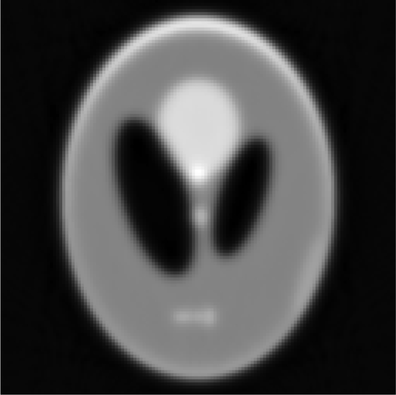
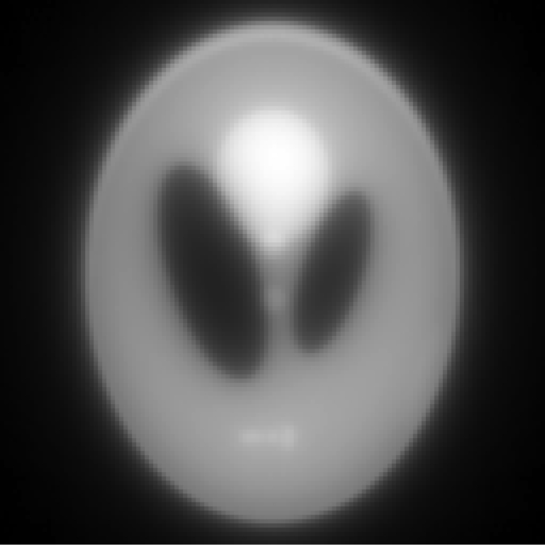
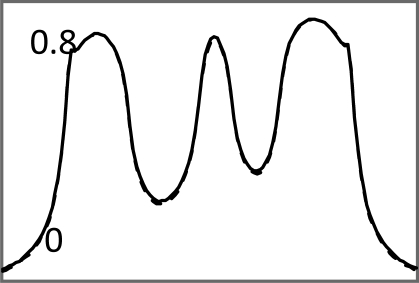
Computer simulation results are shown in Tables 1, 2, 3, 4, 5, TABLE VI.. Each image is displayed from its minimum image pixel value (black) to its maximum image pixel value (white). No post processing of the images was performed. The negative values in the images were not altered.

TABLE I.

Iterative MAP vs FBP-MAP with β = 0.1 (i.e., small Bayesian term weighting) using noiseless data.

	Iteration index k = 2	k = 20	k = 200
Iterative result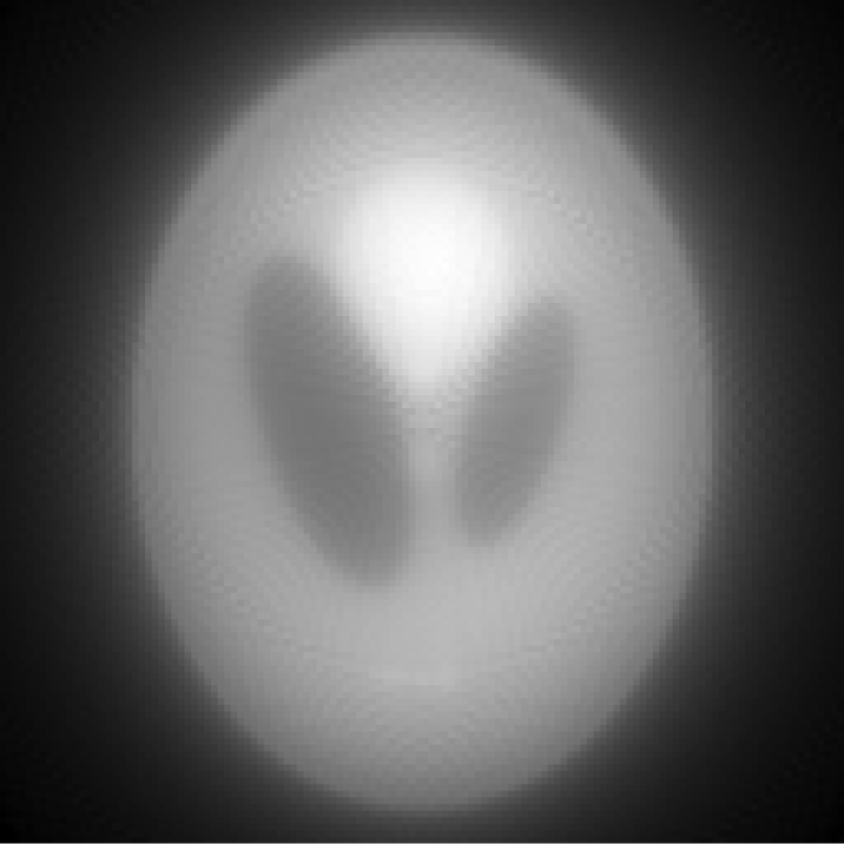
FBP result
Central horizontal profiles (vertical scale is from 0 to 250)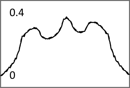

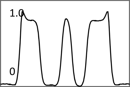TABLE II.

Iterative MAP vs FBP-MAP with β = 0.3 using noiseless data.

	Iteration index k = 2	k = 20	k = 200
Iterative result
FBP result
Central horizontal profiles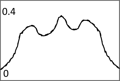

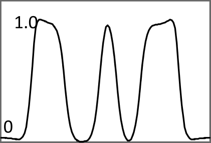TABLE III.

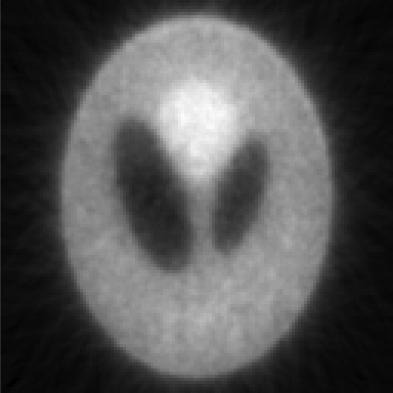
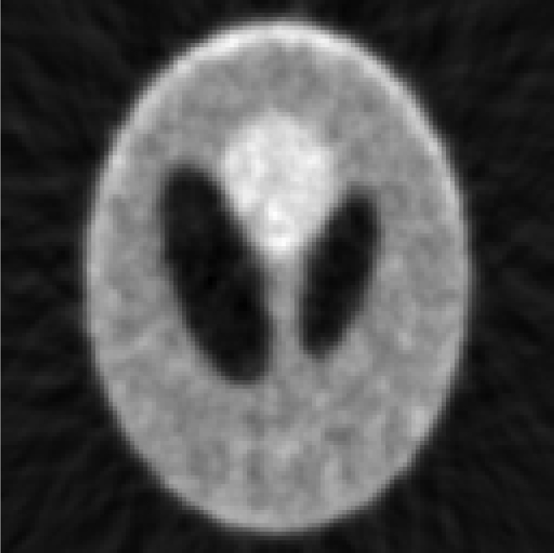
Iterative MAP vs FBP-MAP with β = 0.1 (i.e., small Bayesian term weighting) using noisy data.

	Iteration index k = 2	k = 20	k = 200
One iterative reconstruction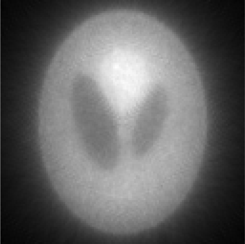
One FBP reconstruction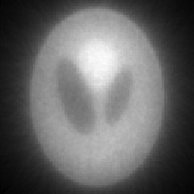
S/N image from 100 noise realizations of iterative reconstructions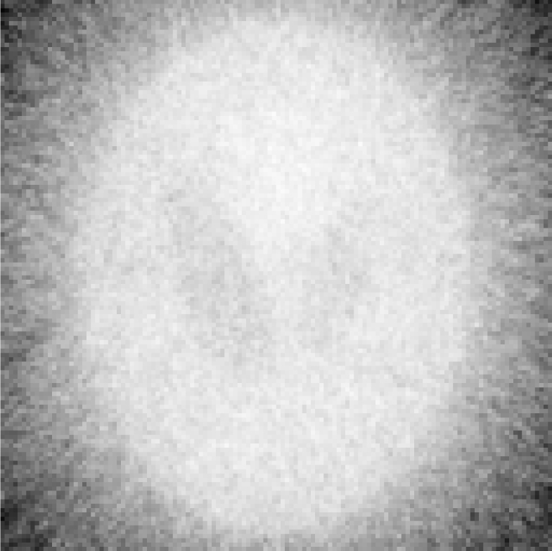
S/N image from 100 noise realizations of FBP reconstructions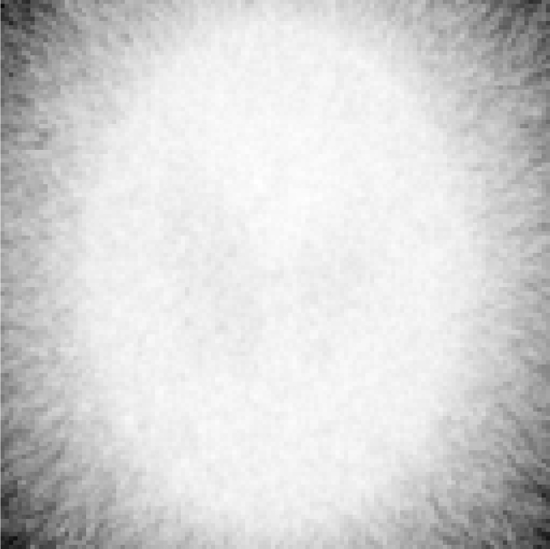
Central horizontal profiles of the S/N images (vertical scale is from 0 to 250)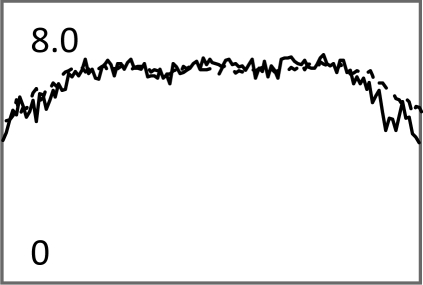

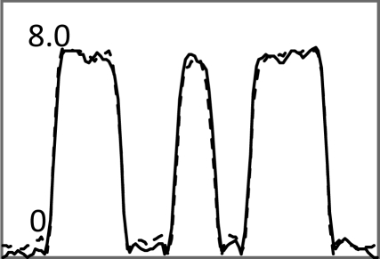TABLE IV.

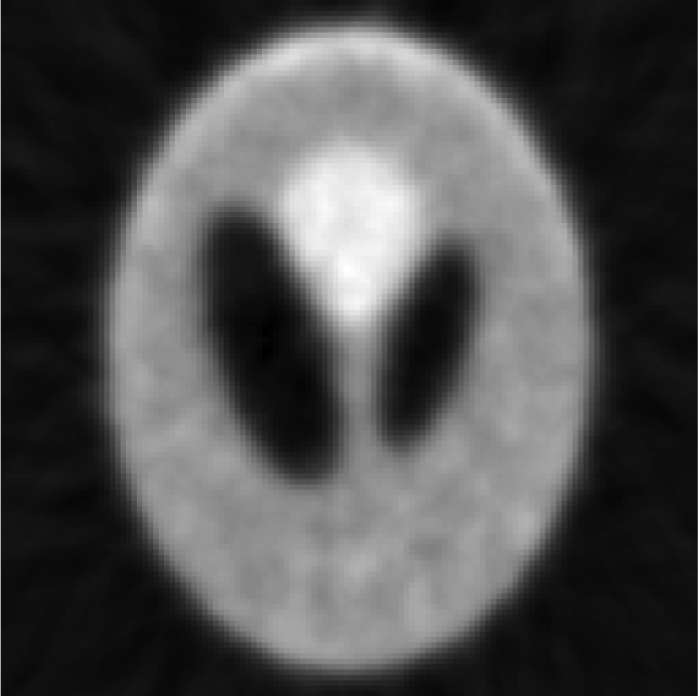
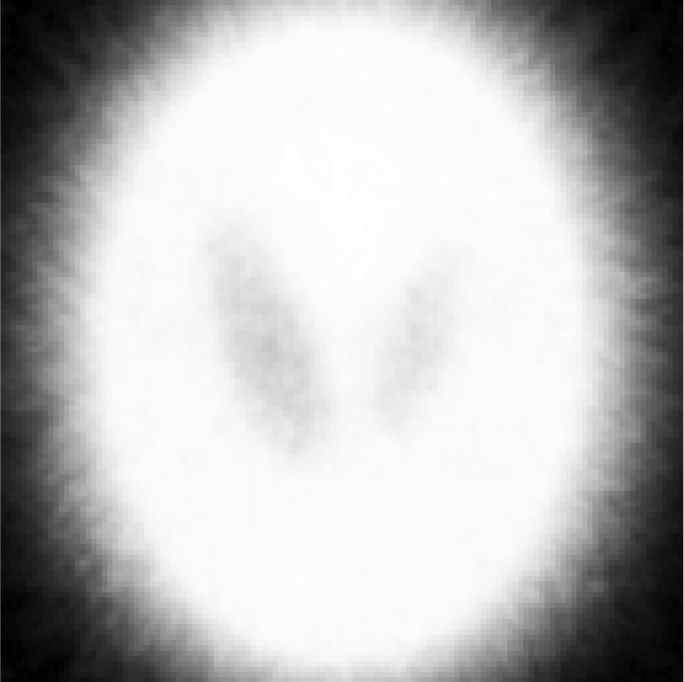
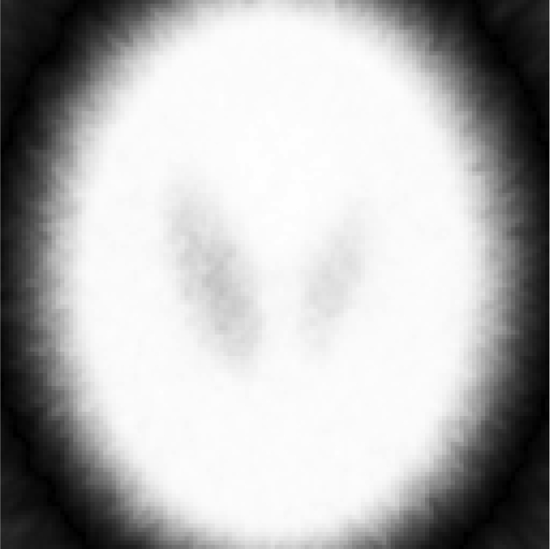
Iterative MAP vs FBP-MAP with β = 0.3 using noisy data.

	Iteration index k = 2	k = 20	k = 200
One iterative reconstruction
One FBP reconstruction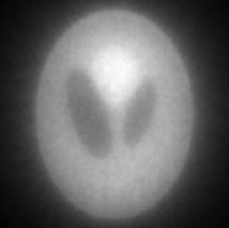
S/N image from 100 noise realizations of iterative reconstructions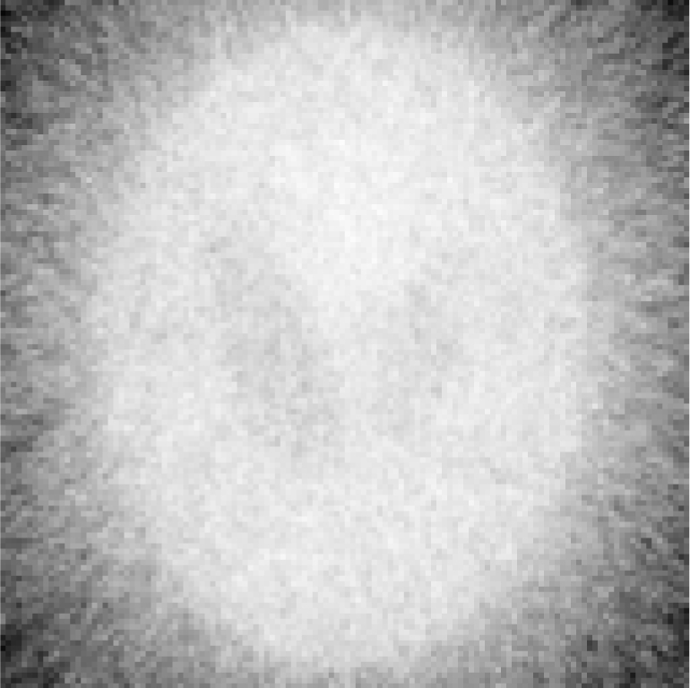
S/N image from 100 noise realizations of FBP reconstructions
Central horizontal profiles of the S/N images (vertical scale is from 0 to 250)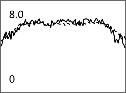

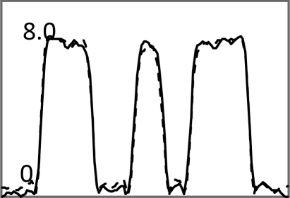TABLE V.

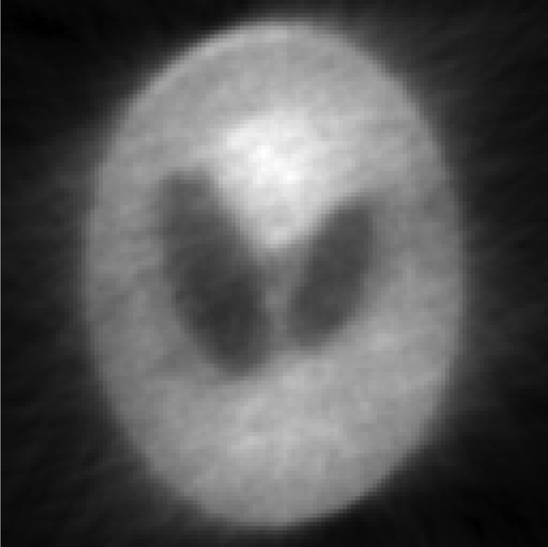
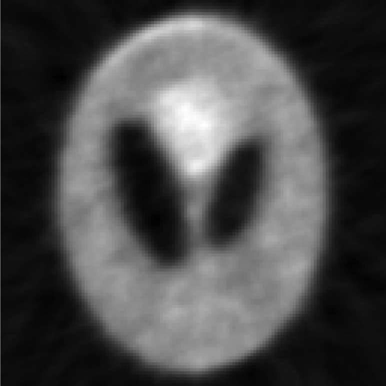
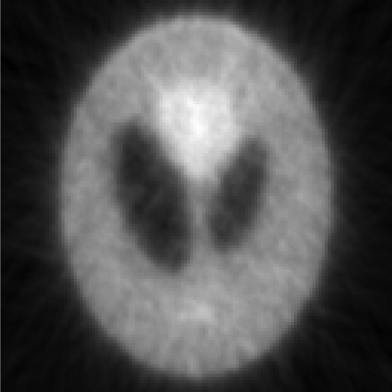
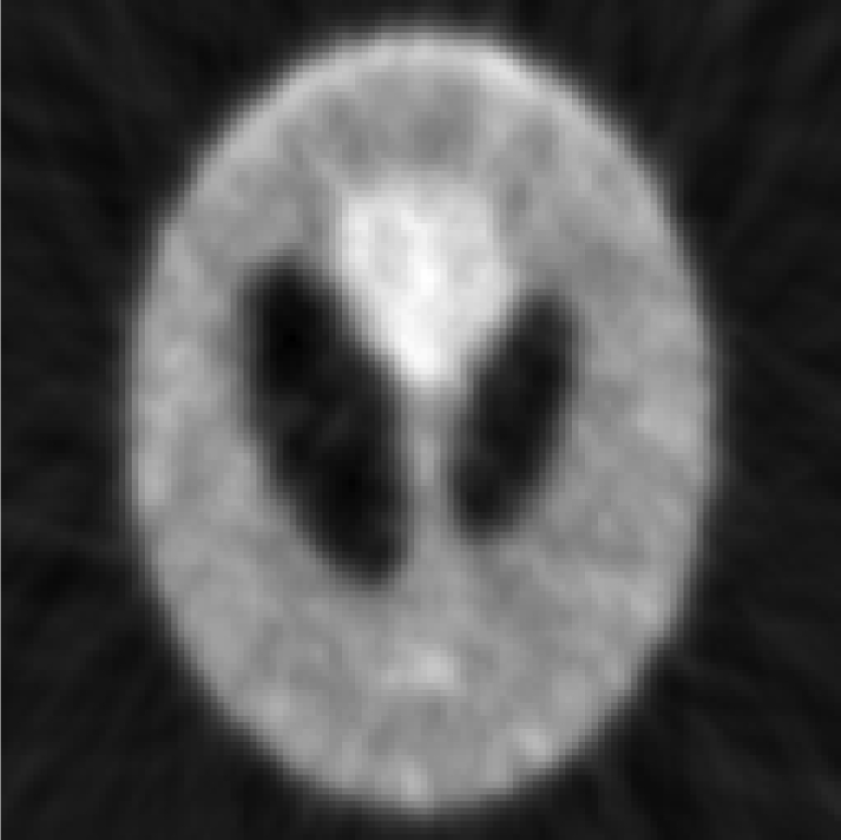
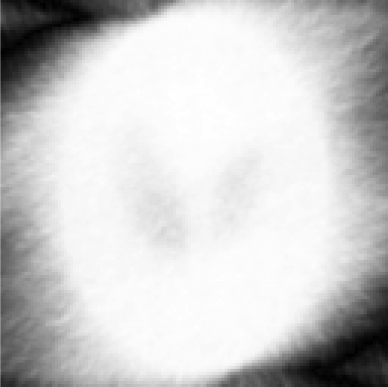
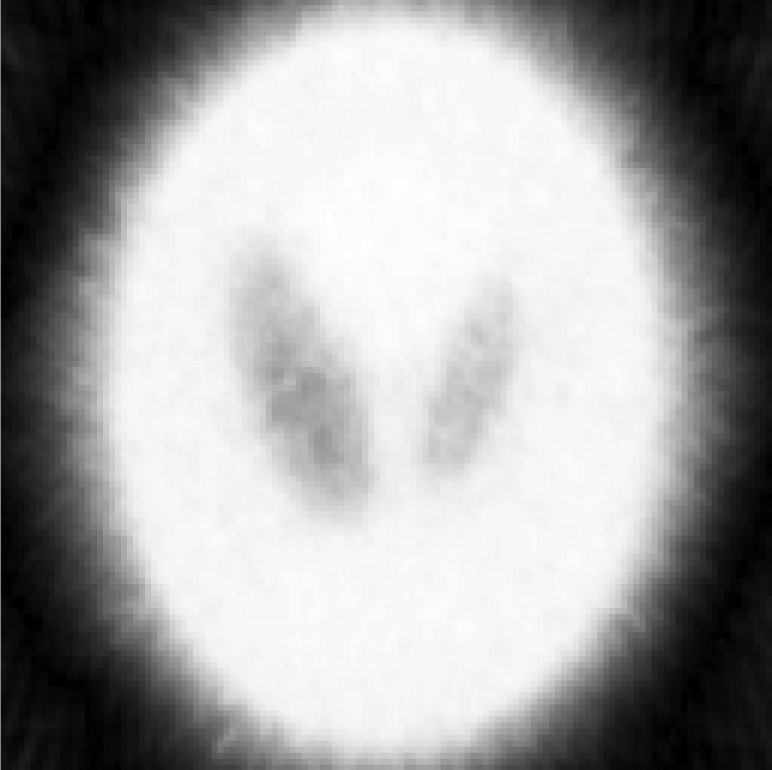
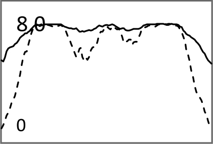
Iterative MAP vs FBP-MAP with β = 0.3 using nonuniform angular sampling (noisy data).

	Iteration index k = 2	k = 20	k = 200
One iterative reconstruction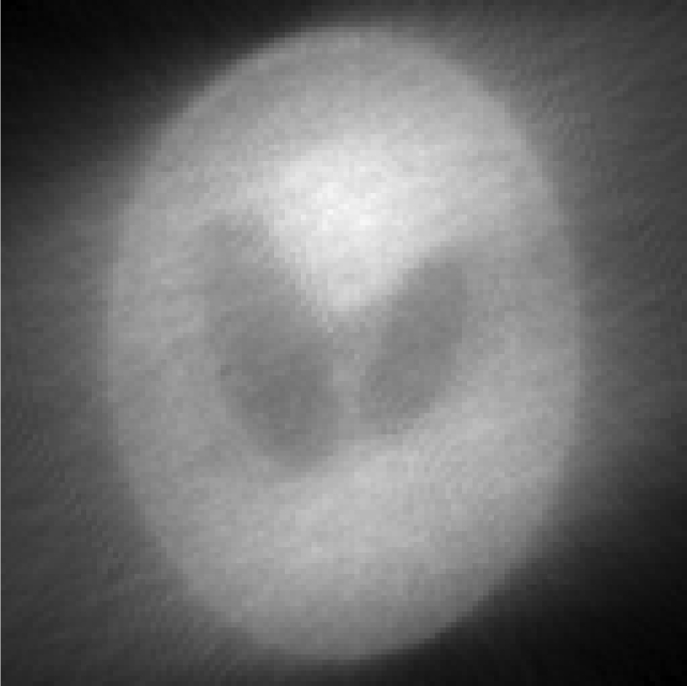
One FBP reconstruction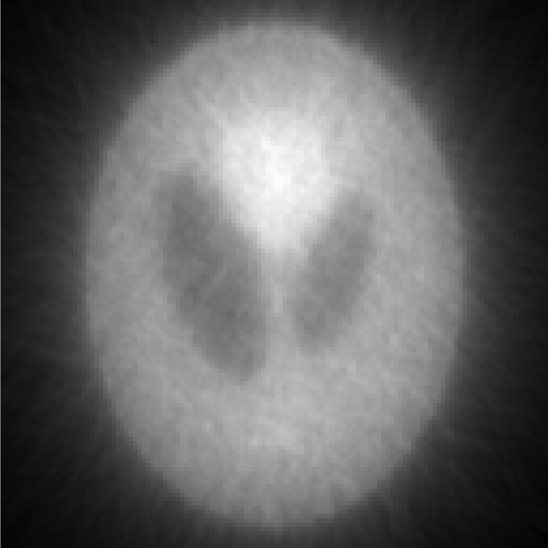
S/N image from 100 noise realizations of iterative reconstructions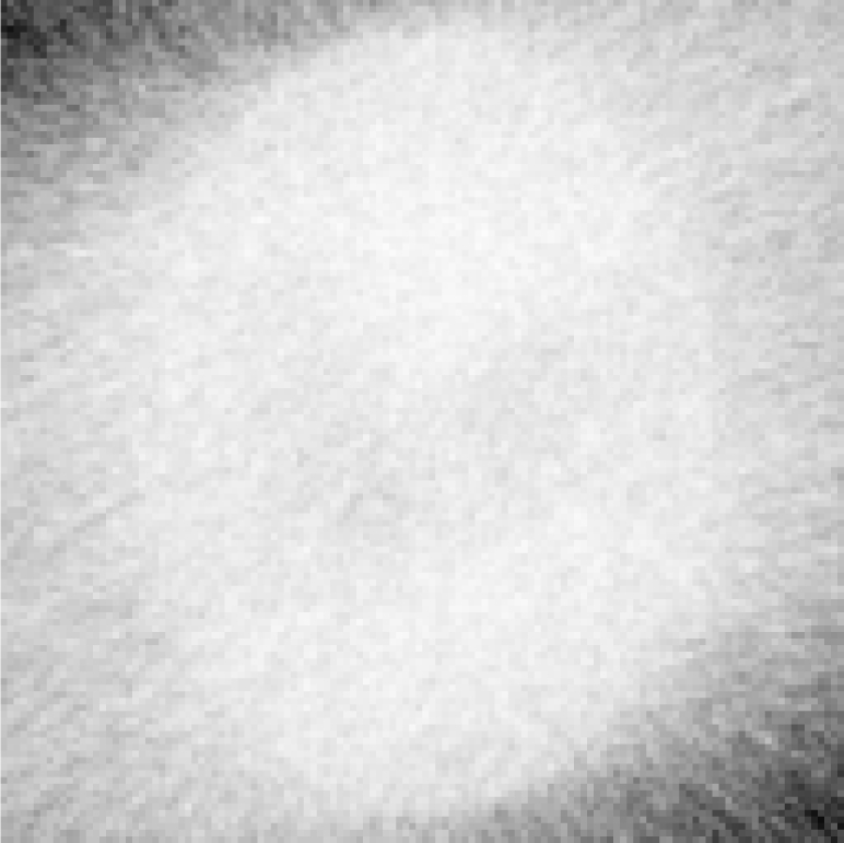
S/N image from 100 noise realizations of FBP reconstructions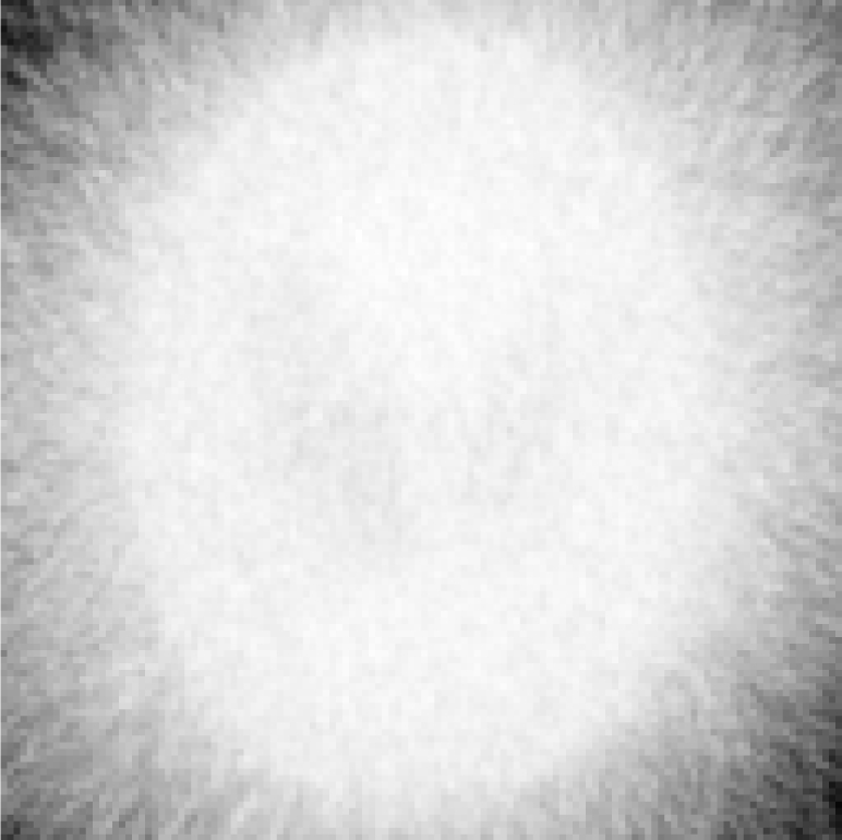
Central horizontal profiles of the S/N images (vertical scale is from 0 to 250)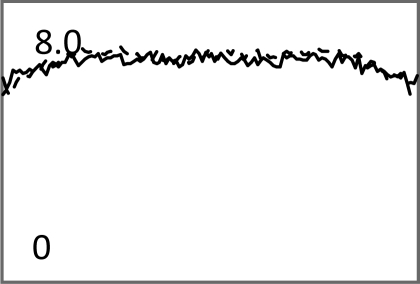

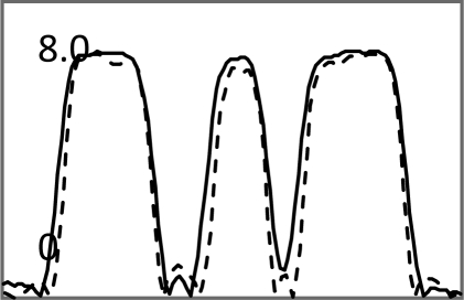TABLE VI.

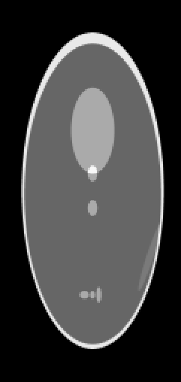
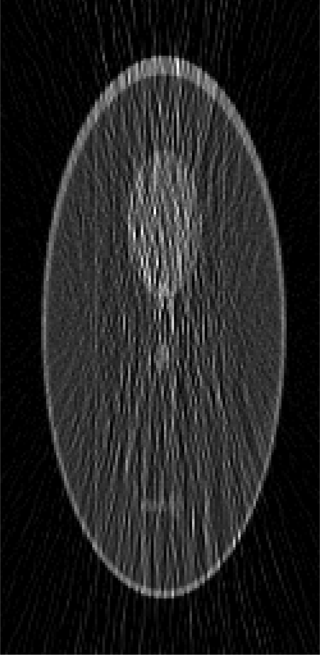
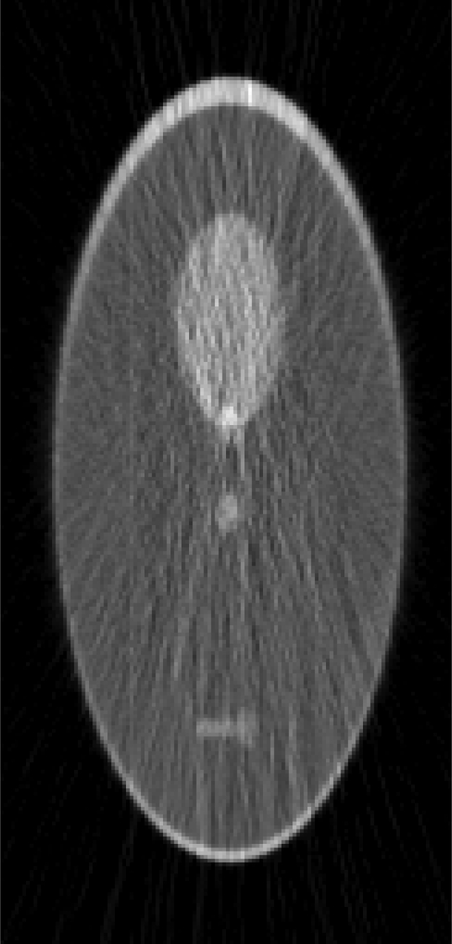
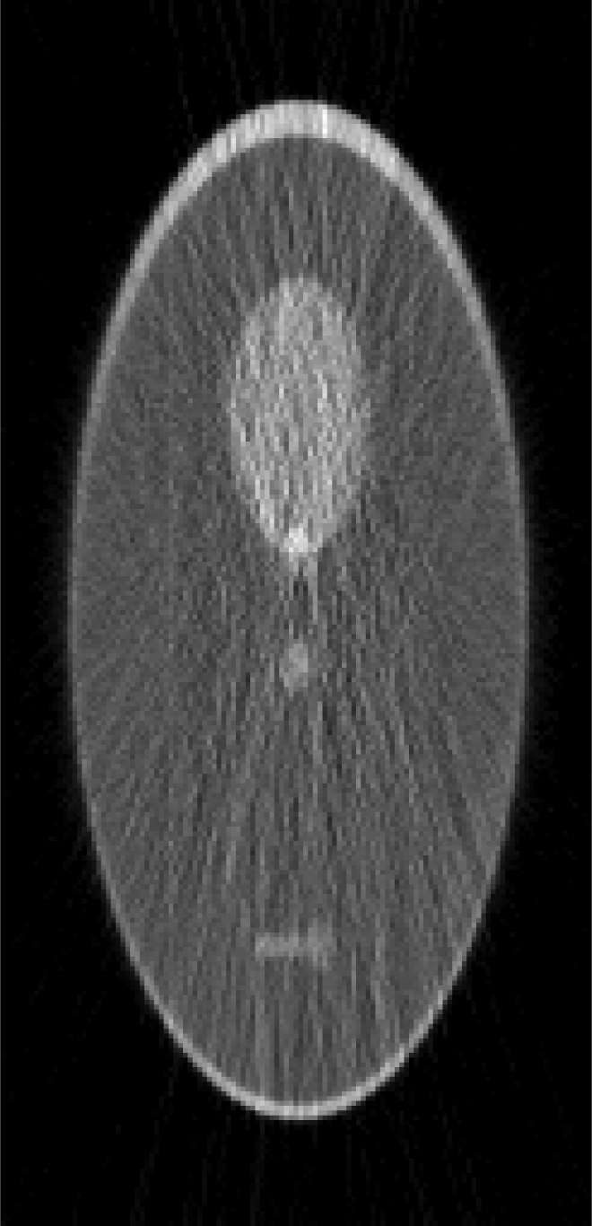
Computer simulations for low-dose CT

True phantom	Regular FBP (k = ∞)	View-wise noise weighted FBP (k = 64)	Iterative Landweber with view-wise noise weighting (k = 64)	Iterative Landweber with ray-wise noise weighting (k = 739)
MSE = 0	MSE = 3.9	MSE = 0.85	MSE = 0.91	MSE = 1.17

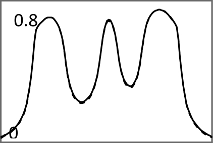
Images in Tables 1, TABLE II. used noiseless projections, and they are used to illustrate the resolution improvement as the index k gets larger. The profiles are drawn horizontally at the center of the images. The images almost converge when k = 200. From the profiles, one can tell that a larger β value makes the image smoother. With the same index k, the iterative Landweber MAP algorithm and the windowed FBP algorithm give almost the same resolution.

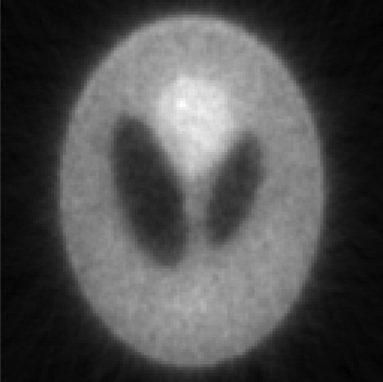
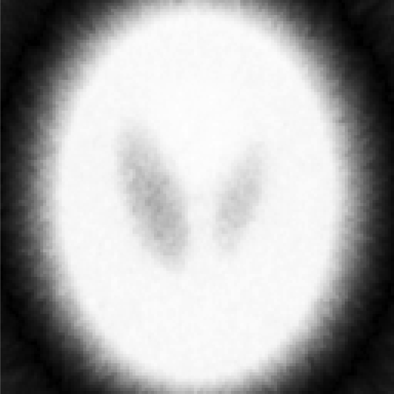
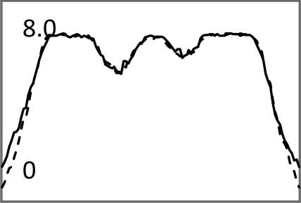
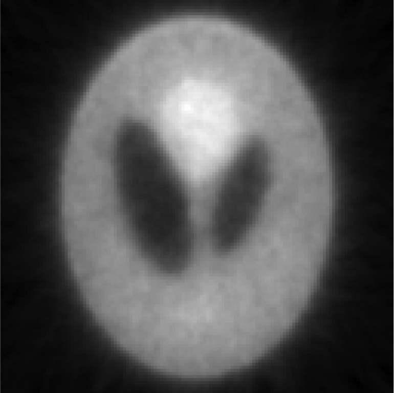
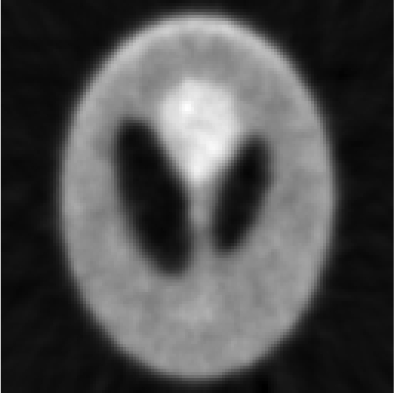
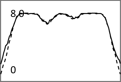
In Tables 3, TABLE IV., Poisson noise was added to the projections. Typical reconstructions are displayed in the rows 2 and 3. As the index k increases, the resolution improves, but the noise is amplified. Signal-to-noise (S/N) ratio images were obtained by using 100 noise realizations and are displayed in the 4th and 5th rows. In the S/N image each pixel represents the ratio of the mean value over the standard deviation. As shown by the line profiles drawn horizontally across at the center of the S/N images, the iterative Landweber MAP algorithm and the proposed FBP algorithm have almost the same noise property for the same index k.

Nonuniform angular sampling

In Table TABLE V., the angular sampling was nonuniform. The sampling interval was 1° for $0\le \theta <\pi /4$ and 3° for $\pi /4\le \theta <\pi$; the density function is given in Eq. 10. One can observe many differences between the iterative results and the FBP results: In early iterations, the results of the iterative MAP algorithm contain 45° directional blurring due to the nonuniform angular sampling effect. The FBP-MAP algorithm does not have this artifact.

Noise weighted FBP

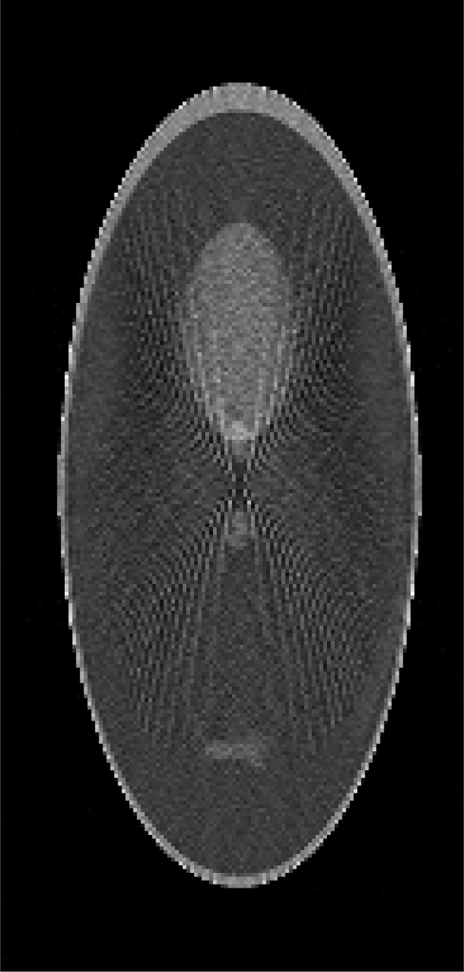
In this section, an example that simulates low-dose transmission x-ray CT is provided. When the object shape is elongated, streaking artifacts are most likely to appear in the direction of the longest dimension. In order to show the streaking artifacts, the Shepp-Logan phantom was modified and elongated. First, the projection data p were generated analytically as line-integrals of the phantom. Second, transmission data N = N₀e^−p were formed with incoming flux N₀ = 8000. Third, Poisson noise was added to the transmission data N. Forth, the noisy transmission data (N + Poisson noise) were transformed to noisy line-integrals to be fed to image reconstruction algorithms by p = ln[N₀/(N₀e^−p + Poisson noise)]. In the noise weighted FBP algorithm, the noise variance can be modeled as 1/N. For every projection view, the weighting factor was chosen as w_view = (N_central/N₀)^0.2, with N_central being the noisy transmission measurement of the central ray on the detector. The power 0.2 was selected so that a smallest mean-square-error (MSE) between the reconstruction and the true image can be achieved.

An iterative Landweber algorithm (which is the same as Eq. 2 except that A^T is replaced by A^TW and β = 0) was implemented to include the view-wise noise model w_view = (N_central/N₀)^0.2 and used to reconstruct the image with the same data. The stopping rule, i.e., the criterion of selecting parameter k, is that the MSE between the reconstruction and the true image reaches the minimum. It is clear that this stopping rule can only be applied to computer simulations, because the true image is not known for any practical applications. The reconstruction results are shown in Table TABLE VI.. It is seen that the weighted FBP algorithm and the weighted iterative Landweber algorithm give almost the same reconstruction.

Table TABLE VI. also shows a reconstruction using the weighted iterative Landweber algorithm in which the ray-based (instead of view-based) noise weighting is used and the weighting function is w_ray = (N_ray/N₀) without the power of 0.2. This weighting scheme is widely accepted in imaging community as the accurate weighting method. It seems that using the reciprocal of the noise variance as the weighting factor may not always be optimal and the optimal weighting strategy still needs further investigation.

CONCLUSIONS

This paper derived an FBP-MAP algorithm that has a window function with an index k that can emulate the iterative Landweber MAP algorithm of the kth iteration. Computer simulations show that the FBP-MAP algorithm and the iterative MAP algorithm give very similar images and noise texture if they have the same index k, same parameter α, and same parameter β. The most significant advantage of the FBP-MAP algorithm is its fast computation time; the iterative MAP algorithm is 2k times slower. Another advantage of the FBP-MAP algorithm is that it has a shift-invariant point-spread-function (i.e., uniform resolution). On the other hand, the iterative algorithm has a nonuniform resolution convergent rate.

When the sampling is nonuniform, the new FBP algorithm is able to compensate for it using a normalization factor. While nonuniform sampling is not a main concern in an iterative algorithm, in early iterations, the nonuniform sampling may introduce some directional nonuniformity artifacts.

To our knowledge, noise modeling has never been considered in an FBP algorithm before. This paper first incorporates view-based noise model in the FBP algorithm. This noise model may find applications in low-dose x-ray CT imaging.

The methods introduced in this paper can be extended to the cone-beam imaging geometries. For the circular-orbit cone-beam imaging, Feldkemp’s FBP algorithm¹² can be modified by window functions. For the spiral-orbit cone-beam imaging, Katsevich’s FBP algorithm¹³ can be modified by window functions. This paper is only an initial investigation, many problems are yet to be solved, such as ray-based projection noise modeling, nonideal projection geometry, nonstationary resolution effects, very sparse data sampling, as well as a general Bayesian term that cannot be expressed as a convolution or a quadratic form. All these challenges will be met in our future investigations.

References

- Shepp L. A. and Logan B. F., “The Fourier reconstruction of a head section,” IEEE Trans. Nucl. Sci. NS-21, 21–43 (1974).
- Xu X.-L., Liow J.-S., and Strother S. C., “Iterative algebraic reconstruction algorithms for emission computed tomography: A unified framework and its application to positron emission tomography,” Med. Phys. 20, 1675–1684 (1993). 10.1118/1.596954 [DOI] [PubMed]
- Strand O. N., “Theory and methods related to the singular-function expansion and Landweber’s iteration for integral equations of the first kind,” SIAM (Soc. Ind. Appl. Math.) J. Numer. Anal. 11, 798–825 (1974).
- Zeng G. L., “A filtered backprojection algorithm with characteristics of the iterative Landweber algorithm,” Med. Phys. 39, 603–607 (2012). 10.1118/1.3673956 [DOI] [PMC free article] [PubMed]
- Wang C. X., Snyder W. E., Bilbro G., and Santago P., “Performance evaluation of filtered backprojection reconstruction and iterative reconstruction methods for PET images,” Comput. Biol. Med. 28, 13–25 (1998). 10.1016/S0010-4825(97)00031-0 [DOI] [PubMed]
- Geman S. and McClure D. E., “Statistical methods for tomographic image reconstruction,” Bull. Internat. Statist. Inst. LII-4, 5–21 (1987).
- Levitan E. and Herman G. T., “A maximum a posteriori probability expectation maximization algorithm for image reconstruction in emission tomography,” IEEE Trans. Med. Imaging 6, 185–192 (1987). 10.1109/TMI.1987.4307826 [DOI] [PubMed]
- Green P. J., “Bayesian reconstruction from emission tomography data using a modified EM algorithm,” IEEE Trans. Med. Imaging 9, 84–93 (1990). 10.1109/42.52985 [DOI] [PubMed]
- Cao G., Bouman C. A., and Webb K. J., “Noniterative MAP reconstruction using sparse matrix representations,” IEEE Trans Imaging Process. 18, 2085–2099 (2009). [DOI] [PubMed]
- Schafer R. W., Mersereau R. M., and Richards M. A., “Constrained iterative restoration algorithms,” Proc. IEEE 69, 432–450 (1981). 10.1109/PROC.1981.11987 [DOI]
- Zeng G. L., Medical Image Reconstruction, A Conceptual Tutorial (Springer, Beijing, 2010).
- Feldkamp L. A., Davis L. C., and Kress J. W., “Practical cone beam algorithm,” J. Opt. Soc. Am. A 1, 612–619 (1984). 10.1364/JOSAA.1.000612 [DOI]
- Katsevich A., “Theoretically exact filtered backporjection-type inversion algorithm for spiral CT,” SIAM J. Appl. Math. 62, 2012–2026 (2002). 10.1137/S0036139901387186 [DOI]