

Abstract
Purpose
To evaluate whether MR thermometry is sufficiently fast, accurate, and spatially resolved for monitoring the thermal safety of non-ablative pulsed HIFU (pHIFU) treatments.
Materials and Methods
A combination of real MR thermometry data and modeling was used to analyze the effects of temporal and spatial averaging as well as noise on the peak temperatures and thermal doses that would be measured by MR thermometry.
Results
MR thermometry systematically underestimates the temperature and thermal doses during pHIFU treatment. Small underestimates of peak temperature can lead to large underestimates of thermal dose. Spatial averaging errors are small for ratios of pixel dimension to heating zone radius less than 0.25, which may be achieved by reducing the voxel size or steering the acoustic beam. Thermal dose might also be underestimated for very short, high power pulses due to temporal averaging. A simple correction factor based on the applied power and duty cycle may be applied to determine the upper bound of this effect.
Conclusion
The temperature and thermal dose measured using MR thermometry during pulsed HIFU treatment is probably sufficinet in most instances. Simple corrections may be used to calculate an upper bound where this is a critical factor.
Keywords: pulsed high intensity focused ultrasound, HIFU, drug delivery, ultrasound hyperthermia, MR thermometry
INTRODUCTION
Focused ultrasound is a technology whereby ultrasound energy from a large transducer (or transducer array) is concentrated into a very small volume, where it deposits significant thermal and strain energy into the tissue. This technology has already gained some clinical acceptance as a means of thermally ablating soft tissues (1, 2, 3). Potential non-thermal therapies are also being considered in a number of preclinical studies. This relies on the strategy of pulsing of the ultrasound beam with a low duty cycle to allow heat to dissipate, while still maintaining high peak powers during the active part of the cycle. One of the more commonly discussed applications for pulsed high intensity ultrasound (pHIFU) is for enhanced local drug delivery. This might be accomplished by applying methods that enhance the diffusion of large molecular weight drugs and nanoparticles through endothelial and tissue barriers with or without the assistance of intravascular microbubbles (4–11). Alternatively, pulsed ultrasound might be used to deploy drug from a nanocarrier (12,13) or microbubble (14). Other potential uses of pHIFU include mechanical ablation (15,16), or gene upregulation (17,18). Similar technology might be useful for producing controlled local hyperthermia without inducing thermal damage (19). With the exception of this last, all of these applications have in common the preference of mechanical rather than thermal energy, and thus pulsing is a necessity. Even with a reduced duty cycle, however, avoiding significant tissue heating can be a major challenge. MR thermal imaging would appear to be an ideal method for ensuring the safe and effective application of pHIFU under clinical conditions. The near real time feedback, non-invasive nature, and full field imaging of MR thermometry has already made it a standard measurement technique for a multitude of heat producing technologies, including ultrasound, laser, microwave and RF ablation (20,21). In clinical applications, MR thermometry is an integral part of the ExAblate® system (InSightec, Inc., Haifa, Israel), the only HIFU ablation system currently approved for clinical use in the United States, as well as other systems awaiting FDA approval. It is an obvious step to convert this technology, designed for ablation, to be used in drug delivery or hyperthermia applications with pHIFU. It is less clear whether the MR thermometry is up to the challenge of safely monitoring pHIFU treatment. While it is well established that MR thermometry is sufficiently accurate for monitoring tissue thermal necrosis (1,22), the requirements for preventing thermal damage are more stringent, and addressing the safe use of MR thermometry for non-ablative treatments is an important challenge. Maintaining a low thermal dose is not a trivial issue, even with reasonably accurate real-time temperature monitoring, because tissue inhomogeneity and vascularity can affect heating and cooling times in difficult to predict ways (23). Furthermore, the power-law dependence of the thermal dose on temperature can result in a rapidly fluctuating thermal dose for even mild changes in temperature (24). The typical measurement method, using the proton resonance frequency shift (PRF), does not work in adipose tissue, and is sensitive to susceptibility and motion artifacts (20). Although there are now various proposals to correct for these issues (25,26), they have yet to be widely implemented. As well, limitations in temporal and spatial resolution can result in an underestimation of peak temperatures when dealing with rapidly varying temperatures such as those produced by pulsing focused ultrasound (27). In this paper, these issues are approached quantitatively by simulation of the treatment and thermal measurement process. The idea here is not to develop new, or more accurate models of thermal dose, tissue heating, or MR thermometry, but to establish what kind of measurement accuracy one could reasonably expect under the best of circumstances using a clinically relevant system. Our particular interest is in the use of pHIFU for drug delivery in the absence of microbubbles. A typical application of pHIFU for this type of treatment has consisted of 100 or more pulses, at 5 % duty cycle and 1 Hz repetition rate at 40 W peak acoustic power, for each focal spot placed on a grid of 2 mm separation (10,28). More recently, we have also been interested in treatments with longer duty cycles (up to 15 %) and higher power, short duty cycles (≤5%, up to 280 W). These latter are beginning to approach average power deposition levels that can potentially cause thermal damage. The question arose of whether the thermal doses calculated from time-temperature curves, such as those derived by the InSightec system, were sufficiently accurate.
MATERIALS AND METHODS
MR guided Focused Ultrasound System
The ExAblate® 2000 MR guided focused ultrasound device from InSightec, Inc. (Haifa, Israel) was used for all procedures. This device is capable of single and multiple focal spot treatments, where the latter are performed by electronically steering the focal spot in a small region. Here, we use “focal spot” or “focal zone” exclusively in the sense of the physical, diffraction limited focal spot while “treatment zone” refers to a contiguous volume that is treated, potentially with multiple focal spots. “Sonication” is a term that is often used interchangeably with treatment zone, however, it appears to more properly refer to a continuous treatment event, so in our usage, a single treatment zone could potentially receive multiple sonications in multiple passes (4). Anatomical imaging and temperature monitoring is done with a GE 3.0T HDxT magnetic resonance scanner using a breast coil provided by InSightec, Inc. The details of the modifications required to operate this device effectively in pulsed mode are found elsewhere (4). The ExAblate® system uses the proton resonance shift (PRF) technique to measure temperature (29), using a baseline image acquired prior to sonication as a reference. The baseline temperature was always set to be 37 °C. Thermal images were made every 3 s or 9 s, adjusted by modifying the number of averages (NEX) acquired. Nine second thermal maps were used only for sonications lasting longer than 500 s, to avoid long delays in analyzing and transferring MR data to the ExAblate® control PC. During treatment, a coronal slice (perpendicular to the beam) in the focal plane (as calculated by the system) was continuously scanned using a fast gradient echo sequence (echo time 9.4 ms, repetition time 38 ms, flip angle 45, slice thickness 3 mm, FOV 220 mm×220 mm, acquisition, matrix 256×256. The standard pixel spacing for the thermal maps was 0.859 mm×0.859 mm. Magnitude and phase images and temperature maps were automatically reconstructed by the device as is done in clinical practice, and the temperature maps thus obtained were used in the further analysis offline.
In order to operate effectively for pulsed mode HIFU, the ExAblate® control system had to be modified somewhat from the clinical configuration. A non-FDA approved research version of the ExAblate® software was adapted for use in pulsed mode. Pulsed-mode operation was introduced by integrating an external pulser (Agilent, Inc.) to provide a gating signal with the desired pulse width and repetition rate. The ExAblate® system software for cavitation detection was found insufficient for the modified (pulsed) system and therefore, to ensure consistent cavitation detection, the backscattered ultrasound signal from each pulse was fed into an external spectrum analyzer (Agilent, Inc.) triggered by the external gating signal, and the resulting spectrum was stored. Cavitation signatures (high half harmonics, sub-harmonic noise) could generally be eliminated for acoustic powers less than 80 W with improved ultrasonic coupling.
Tissue Measurements
In vivo sonications were done in the thigh muscle of rabbits, in order to provide raw heating data upon which to base our models. All animals were handled according to a protocol approved by the animal care and use committee. Following sedation, the thigh to be treated was shaved and depilated. The shaved leg was placed in a shallow pool of degassed water on a 4.0 cm thick gel pad above the acoustic window of the ultrasound transducer. Degassed water also coupled the ultrasound from the transducer into the gel pad. The gel pad was located at the center of a breast coil (15 cm inner diameter) provided by InSightec, Inc., which was used to acquire MR images of rabbit muscle during treatment. This afforded significantly better signal to noise in the region of treatment than the standard body coil typically used during clinical operation for uterine fibroid treatments. MR thermometry was used to obtain temperature maps during treatment as described in the previous section. Treatments in rabbit muscle tested the heat build-up and dissipation during single sonications, using 100–500 pulses with duty cycles varying for 5 % to 25 %, at 40 W, 1.0 MHz center frequency and 1 Hz repetition rate. The heat build-up in the treatment zone was captured by MR thermometry.
Analytical Modeling and Fitting
The thermal measurements over space and time were fit to the analytical solution to the Pennes bio-heating equation during pHIFU treatment as derived in (10). Briefly, with the ultrasound beam at the focal plane treated as Gaussian, the bio-heat equation may be written:
| [1] |
where the parameters are defined in Table 1 and r is measured from the center of the acoustic beam. This 2d expression works because the length of the focus (7 mm) is much larger than the beam diameter (1.5 mm), so virtually all thermal diffusion is in the plane, not only right at the center of the focal zone (z=0), but also for several mm towards either end (|z|<focal diameter). Since our slices are taken in the coronal direction perpendicular to the beam axis, and the thickness of 3 mm is less than half the length of the focal zone, the 2d thermal model is appropriate here, and it should be noted that voxel averaging out of the plane is also insignificant, as demonstrated in (27). While the pulse is active, the final term dominates. That is, we can write the active solution like:
| [2] |
The additional term, a1t, used here compared to (10) allows us to consider longer duty cycles. Taking the derivatives of [2] in space and time, and dropping terms of order t2, r2 and larger, we arrive at:
| [3] |
from which and , with . Based on this, following the end of the nth pulse at time tn=n(Δton+Δtoff)−Δtoff, the decay is as in (10):
| [4] |
where . This expression was implemented Python/SciPy (30) code to simulate a single sonication pHIFU treatment. The simulation results were fit to the measured temperature field over time using the SciPy least squares (leastsq) fitting routine to find , B, ω, R, the ambient temperature with a drift term, Ta=T0+Ct, and the location (x0,y0) of r=0. The necessity of drift term was particularly evident in some of the longer sonication of 500 s or more and may reflect either actual temperature changes or magnet phase drift. As well, the fit was weighted according to exp(−0.01r2/mm2) to reduce the impact of the more abundant, noisy data at large radial distance and enhance the more important data near the peak of the treatment. The accuracy of the fit was estimated by looking at the residual unexplained variance ( not to be confused with the beam radius, R) after taking into account the deviation of the data from the fit and the inherent noise, that is, we looked at:
| [5] |
where is the variance of the residuals (square deviation of the data from the fit), is the total variance of the data (square deviation of the data from zero), and is the variance of the noise (square deviation of the data in the absence of any perturbation). This last value was measured from the thermal map at the earliest possible time point, presumably before any significant heating had occurred. The alternative is to use literature sources or manufacturer specifications for noise estimates. The use of this unconventional expression allows us to retain the simplicity of the commonly used coefficient of determination, which approaches unity as the fit gets progressively better, while addressing the issue of known measurement noise. That is, a “perfect fit” of in this case implies the deviation from the fit is just noise. Certain physical parameters were assumed, including the tissue heat capacity, c, and density, ϱ, and the peak acoustic power given by the device. An arbitrary level of was used as an objective means to eliminate treatments that, for one reason or another, contained systematic errors such as motion or susceptibility artifacts. Based on the fitted parameters extracted from sonications of various lengths and duty cycles on multiple animals, we were then able to extract the remaining physical parameters, k and α, for comparison with literature. We also extracted, as a fitted parameter, the half maximum radius of the beam, , which was not assumed to be the −3 dB radius of the ExAblate focal zone as measured in water by InSightec.
Table 1.
Fitted parameters
| Parameter | Definition | Value (Standard Dev.) |
|---|---|---|
| Fixed Parameters | ||
|
| ||
| c | tissue heat capacity | 3600 J/kg°C |
| ϱ | tissue density | 1050 kg/m3 |
|
| ||
| Direct Fit Parameters | ||
|
| ||
| ω | blood perfusion time constant | 0.007(0.01) Hz |
| R | beam width | 1.6(0.4) mm |
| k | tissue thermal conductivity | 0.7(0.2) W/m°C |
|
| ||
| Derived Parameters (based on Power) | ||
|
| ||
| α | ultrasonic absorption | 2.6(0.6) Np/m |
Thermal Dose Simulations
Based on the fitted parameters, a hybrid pHIFU model was implemented in a finite element package, Comsol Multiphysics® 4.0, in order to model multiple sonication treatments. With this model, the heat transfer was solved by the finite element method based on the bioheat equation in a 2d approximation. The 2d approximation was done primarily to maintain consistency with the previous 2d analytical fit. The “tissue” was a homogeneous block 80 mm wide by 80 mm long, with the treatment zone at the center. External tissue heating was applied assuming absorption of energy from a Gaussian ultrasonic beam, as in [1]. Tissue and physical parameters (see Table 1) were based on the results of the previously mentioned analytical fit. With this model, first, the numerical and analytical solutions were compared for a single sonication to demonstrate their equivalence, second, the pulsed solution was compared to the result of continuous heat deposition at the same average rate to demonstrate that the loss of temporal resolution does not affect the spatial resolution, and finally, a multi-sonication treatment was simulated using continuous heat deposition. This latter approach was taken because using pulsed heat deposition in the simulations requires much smaller time steps, and therefore much greater computer time, and storage, and also because MR thermometry has no resolution on the scale of individual pulses. Thus, the analysis was broken up into issues of temporal resolution, which were addressed using the single sonication pulsed treatment models, and spatial resolution, which were addressed with the multiple sonication, time-averaged continuous treatment models.
Simulations were used to look at the impact of spatial and temporal averaging on measured peak temperatures and thermal dose. Spatial averaging was carried out within each (isotropic) pixel using the weighting function described in (27):
| [6] |
where δ is the both length and width of each pixel, and the image is N×N pixels. The location of the pixel being imaged is (xi,yj). For simplicity in applying to discreet data, this expression was truncated at the edge of the pixel, and the normalization adjusted accordingly. No weighting was used for the temporal averaging, which was performed over the full acquisition time (3 s).
Thermal dose is often written in terms of “equivalent minutes at 43 °C” as (31):
| [7] |
where R=4 for 37<T<43, and R=2 for T>43. Spatial volume averaging in an MR thermal map has the effect of smoothing the peaks and valleys of any sharply varying thermal field. In our case, this means a systematic underestimation of the peak temperature produced by the pHIFU treatment. To look at the impact of spatial averaging and noise, continuous deposition was used to compare single and multiple focal spot simulations, after first comparing the spatial extents of pulsed and continuous treatment of equal average power for a single focal spot. The simulation data was sampled with a resolution of 1.2 mm, which is close to the beam diameter; as well, Gaussian noise was added with a standard deviation of ±0.3. This noise level is in line with values measured during actual in vivo sonications (to be used in (5)) as well as those communicated from InSightec. The measured temperatures and thermal doses after sampling and noise were then compared back to the simulated high resolution data to draw some conclusions about the inherent accuracy of the measurement process. The same method was used to determine the effects of sampling for a multi-point simulation (9 points treated consecutively, placed on the corners and midpoints of a 4 mm by 4 mm square).
The low temporal resolution of the measurement may also have an impact, particularly, on thermal dose calculations. This problem arises because higher temperatures contribute more to the overall thermal dose than lower temperatures. If one assumes that the MR thermal maps reflect the temporal average temperature, then the reality is that almost half the time is spent at temperatures greater than the measured average, and this contributes more to the thermal dose than the half spent at lower temperatures. Therefore, the thermal dose calculated based on the temporal average is an underestimation by some factor that increases with shorter duty cycle and increasing power. A peak thermal dose correction for a single pulse was derived as follows. For a single pulse near equilibrium, assuming T(t)<43 °C, the thermal dose is:
| [8] |
where:
| [9] |
| [10] |
t1=ton, t2=ton+toff is the repetition period, and ΔT, the distance between peak and valley, is roughly constant near equilibrium. After some manipulation,
| [11] |
Here is the average thermal dose; ΔT is the temperature differential between neighboring `peaks' and `valleys'that may be inferred from the temperature rise during the active part of the duty cycle as , and, as in [7], N=4 for temperatures under 43 °C and N=2 for temperatures above 43 °C. Using simulated data, the thermal dose based on the smoothed time-average temperature and the averaged thermal dose corrected by [11] were compared to the thermal dose obtained by numerical integration of [7] using the “actual” temperatures over a single pulse.
RESULTS
Fitting Parameters for Analytical and Numerical Modeling
Figure 1 shows the analytical solution of [4] fit to the in vivo thermal data. We successfully fit the solution in seventeen of twenty different sonications in four animals. The three sonications that were not fit contained obvious motion artifacts. Two additional sonications were eliminated from further consideration because of unacceptably high unexplained variance (). Of the fifteen remaining fits, the average value of was 0.94 with a standard deviation of 0.06. Noise accounted for less than 15 % of the total variance. None of the fit parameters showed a discernible trend with duty cycle, except possibly the thermal constant, T0, and drift, C, which tended to diverge slightly with increasing duty cycle. The thermal constant during these treatments ranged from 37.44 °C to 38.63 °C (0.44 to 1.63 °C above the system defined ambient temperature of 37 °C), with a median value of 38.13 °C. The thermal drift had values ranging from −0.004 °C/s up to 0.021 °C/s, with a median value of 0.004 °C/s. The remaining physical parameters extracted from the data fitting are listed in Table 1, along with their average values and standard deviations. With the exception of ω, all of these parameters were needed to adequately fit the data, and replacing them with literature values had a significant detrimental impact on the unexplained variance. Finally, no correlation is found across sonications within the final set of parameters, suggesting this combination is, in fact, unique.
Figure 1.
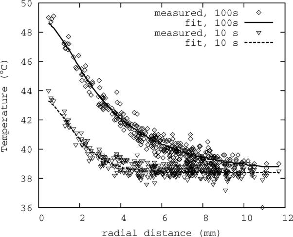
Representative fit of analytical model to thermal data. Shown here are two time points, the lower peak near the beginning of the sonication, and the higher peak near the end. All spatial data is collapsed onto the radial axis for added clarity.
Figure 2 (A) and (B) demonstrate the virtual equivalence of the numerical and analytical solutions at 40 W power, 15 % duty cycle. Figure 3 demonstrates that the overall spatial and temporal behavior of the thermal profile is maintained by using a continuous rather than pulsed application as long as the average power remains the same.
Figure 2.

A: Thermal profile for numerical and analytical (FEM) solutions as function of radial coordinate just before and after the 10th and 100th pulses, and following 125 s. B: Thermal evolution as function of time for numerical and analytical solutions at radial distances of 0, 2, 4, 6, and 8 mm from beam center.
Figure 3.
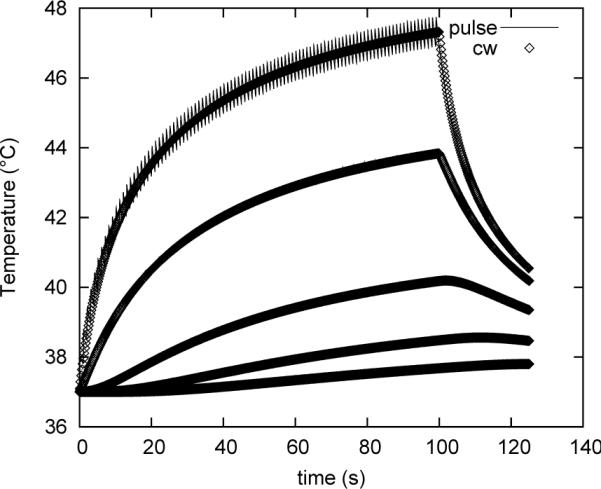
Thermal evolution of pulsed and continuous energy deposition at the same average rate. Pulsing parameters for all plots are: peak acoustic power: 40 W, duty cycle: 15 %, repetition rate: 1 Hz.
Spatial Average Effect on Thermal Dose
In principle, spatial averaging of data around a thermal peak will result in a measurement that underestimates the peak temperature. It is possible to estimate how large this error might be by assuming a Gaussian heating profile and integrating over possible pixel regions in the neighborhood of this beam. If the pixel is centered at (x0, y0) relative to the beam axis, then:
| [12] |
where S(δ)=ΔTM/ΔTP is the ratio of measured peak temperature rise to actual peak temperature rise, δ=fR is the pixel dimension, R is the beam width (related to the radius at half max by ). W is the normalization required to account for the truncation of the integral.
For our typical case, images are 256×256 pixels, and f=δ/R is less than 2. Figure 4 shows how the spatial averaging can affect the measurement of the peak temperature. In particular, from the figure, for f ≈1, , where the lower number comes from having the corner of the pixel at the beam center, and the higher number from having the pixel centered on the beam.
Figure 4.
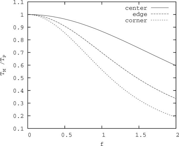
Ratio of measured to actual peak temperature as a function of f, the ratio of pixel dimension to beam radius. Upper curve: beam axis is at the center of the pixel; lower curve: beam axis is at the corner of the pixel; middle curve: beam axis is a middle edge of the pixel.
For pulsed HIFU using the ExAblate® system, the radius of the acoustic beam and thus thermal energy deposition is reported to be 0.75 mm, while the pixel size is 0.895 mm. (In fact, this is made worst by the defaults in the ExAblate software, which reports in real time only the spatial average of the 9 pixels centered on the peak pixel, ostensibly for the purpose of reducing noise. If possible, this feature should be turned off during temperature critical procedures, or it must be taken into account during planning.) Based on Figure 4 it might appear that this should pose a rather large problem. Simulations with the bio-heat equation demonstrate, however, that the width of the thermal profile grows as heat is deposited pulse by pulse (Figure 5), until, at the highest temperatures near the end of the sonication, it has increased in width by over 1 mm.
Figure 5.
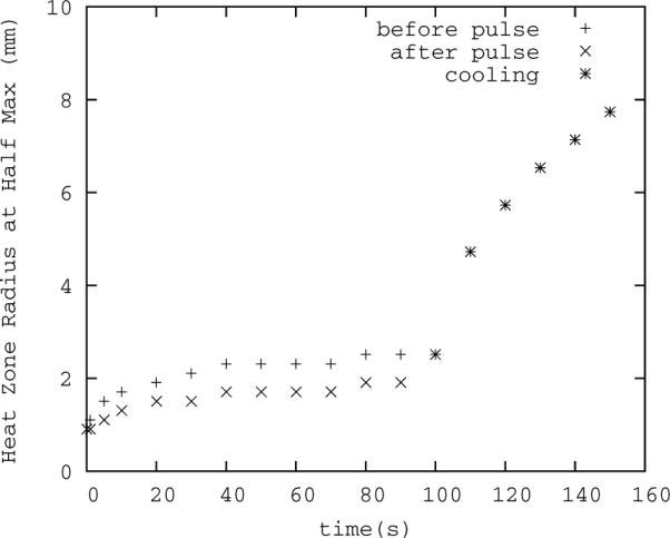
Thermal radius broadening over time. The pulse width is 50 ms, repetition rate is 1 Hz with 100 total pulses, and initial radius 0.75 mm. The lower series of points is the thermal spot size (full width, half max) following the heating portion of the nearest cycle, the upper series is the width following the cooling portion. A larger radius means the average temperature from MR thermometry better approximates the actual peak temperature. The thermal zone width is larger, and therefore measurement error gets smaller, over time and at higher peak temperatures.
Furthermore, our fitting of actual thermal data to the pulsed heating models suggests the beam radius is initially broader in tissue than it is in water. The half maximum radius of the beam may be calculated from our `beam width' parameter, R2, as . Thus, under these conditions, f ≈0.5 and 0.85<ΔTM/ΔTP<0.96. For ΔTM=8 °C, 9.41>ΔTP>8.33 °C. From this, the (temporal average) thermal dose may be estimated using T43≈2ΔT−6°C per pulse at 1 Hz. With ΔTM=8 °C, this gives T43M≈4.0s per pulse, however, from the ΔTP, it implies 10.6 s>T43P>5.0 s per pulse. That is, less than 10 % underestimate in temperature can result in a 50 % underestimate in thermal dose (see Figure 6, middle).
Figure 6.

Effects of coarse sampling and random noise on peak temperature maps and calculated thermal dose for a single treatment zone. The field of view is 20 mm wide. Upper row: peak temperature, lower row: thermal dose. The peak temperature and thermal dose after coarse sampling (pixel width 1.2 mm, middle) are 46.4 °C and 7.5 minutes respectively, somewhat lower than the actual values (left) of 47.2 °C and 12.8 minutes. Adding Gaussian noise results in peak values of 47.0 °C and 7.3 minutes (right).
The effect of noise can help to ameliorate this problem to some extent, because in practice, one is interested mostly in controlling maximum temperature over the time of the treatment. In taking the maximum, the noise is effectively added to the measurement, thus for ΔTM=8 °C, ΔTmax≈8.3 °C, so the difference between the measured ΔTmax, and actual ΔTP is that much smaller (see Figure 6, upper right), but this effect depends strongly on the actual noise level. The effect on the measured thermal dose is much smaller, however, since the signal is being integrated over time and thus has contributions from noise in both directions (see Figure 6, lower right).
While these above estimations apply to single focal spot sonications, quite often such spots are combined to form a larger zone of treatment using some sort of fast steering. In the ExAblate® system, this steering is done electronically within a range of ±3 mm. The net effect of this steering is to smear out the heating profile, i.e.. increasing R. The same pixel resolution therefore results in a smaller f and a smaller overall spatial averaging effect (Figure 7).
Figure 7.

Effects of coarse sampling and random noise on peak temperature maps and calculated thermal dose for a treatment zone of 9 consecutively treated spots. Upper row: peak temperature map, lower row: thermal dose. Left: simulated temperature; right: coarse sampling with noise. Even though the acoustic beam radius is nearly the same as the pixel dimension, spatial averaging effects are small because the effective radius of the thermal distribution is much larger.
Temporal Average Effect on Thermal Dose
Looking at Figure 2, it is clearly impossible for MR thermometry (or practically any other readily available technology) to capture the peak temperatures produced by pHIFU. Based on [11], the thermal dose is underestimated because of this fact. The average temperature during the 100th pulse of our simulation is 47.31 °C. On the basis of the temporal average, the thermal dose during this 1 s period is 19.92 s. The actual thermal dose, based on numerical integration is 20.21 s, which suggests the dose calculated from the average is 1.4 % too low. This difference is not too great mainly because the difference between the peak and valley from one pulse to the next is not great, with ΔT=0.856 °C. Applying the correction factor, [11], gives a thermal dose prediction of 20.22 s, which is 0.04 % greater than the actual. However, realistically we cannot measure ΔT directly, so it must be estimated from the input parameters; in this case . The thermal dose prediction in that case is 20.32 s, a 0.5 % overestimate. The thermal dose for the entire pulsed treatment as displayed in Figure 2, from 0 s to 125 s, is 14.73 minutes; for the temporal average continuous treatment, the thermal dose is 14.51 minutes, 1.5 % less than the actual. Applying the same correction factor as above, without worrying about the transition at 43 °C, results in a thermal dose prediction of 14.80 minutes, 0.5 % greater than actual.
While the numbers above for a relatively modest pulse regimen should be reassuring, it is clear that at high powers, pulsing will become more of an issue for borderline (i.e. nearing tissue damage) thermal doses. For example, we have recently been testing high power, short duty cycle pulses for potential drug delivery applications. Applying the same correction factor to simulated 280 W pulsed treatments at duty cycles from 1 to 5 % results in a thermal dose correction ranging from 2–11 % on thermal doses from 0.2 to 4481 equivalent minutes. In particular, for a 4.0 % duty cycle, [11] predicts a 7 % correction on a measured (time averaged) peak thermal dose of 1105 equivalent minutes, resulting in 1182 equivalent minutes. Numerical integration over of the exact solution gives a peak thermal dose of 1171 minutes. How important this additional 60+ minutes of thermal dose actually is will depend on the goal of the treatment. However, applying the correction results in a reliable upper bound on the thermal dose, an important feature when safety is involved.
To implement corrections for both spatial and thermal averaging effects on the thermal dose, the spatial effect on on the measured temperature should be considered first. To do this, some estimate of the thermal peak width (R) must be used along with [12] or Figure 4. This then gives a correction factor to apply to the thermal maps. The peak thermal dose is then calculated based on the spatially corrected temperatures, and finally, the peak thermal dose from this step is corrected for pulsing using [11], with an appropriate estimate of ΔT.
DISCUSSION
In this paper, we have presented considerations to be made for the safety of pHIFU treatments relying on MR thermometry to limit thermal dose. To do this successfully requires a clear understanding of the limitations of the thermal measurement system. Two fundamental limiting factors of applying MR thermometry for pHIFU monitoring are volume and temporal averaging. Numerous papers have discussed the issues of the artifacts, accuracy, and reproducibility of MR PRF thermal imaging in the context of focused ultrasound ablation, and various approaches to solve those issues (20,27). However, for thermal ablation, the only relevant question is whether a region has received enough heat to kill cells. In practice this can be assessed using averaged temperature measurements, confident with the knowledge that the real temperature must be greater than the measured value. With pHIFU, whether for drug delivery or hyperthermia, outright cell killing is something to be avoided. In principle, the peak heating in a single focal zone or during a single pulse must be under-represented by MR thermometry, as averaging smooths out peaks and valleys. However, the rapid changes in temperature during pulsed treatment cannot be followed using practical MR techniques. Therefore, we were interested in the question of whether such a map can be safely used to monitor peak temperatures during pHIFU. To put these factors in context, the HIFU focus of the ExAblate® system (f=1, 0.9–1.4 MHz transducer) is 1.1–1.7 mm in diameter, and is capable of heating tissue at rates above 1 °C per second. At the same time, we are hoping to use this and similar systems at maximum efficiency to treat large volumes, yet maintain control of peak temperatures and thermal doses over several minutes. It is important to know how the limitations of the measurement might affect our treatments and how systematic errors and noise should be addressed.
To address this question, simulations of pulsed heating were carried out. These simulations were based on physical parameters found during a least-squares fitting of in vivo MR thermometry data to an appropriate analytical model rather than relying on literature values. This approach was used mainly because when our simulations were run using literature values the resulting heating profiles looked obviously different from the thermal maps we found during experiment. This may be because the literature values do not reflect reality in our case, or it may be that certain system reported values, such as acoustic power or beam focal width, are not too accurate, or it may be related to our particular use of simplifying approximations. Deriving our own parameters assures us of relevant, consistent results in comparing these simulations to reality later, even though some of our acoustic and thermal parameters are somewhat at odds with the literature. The full width, half maximum value of the beam radius, 1.37±0.3 mm, found from our experimental fit is about double the manufacturer value of 0.75 mm, based, presumably, on water tank experiments. This broadening may be related to a number of factors, including scattering effects during propagation through muscle layers, or possibly the energy deposition of a real beam with sidelobes and other effects that are not fully captured by a Gaussian model. What is clear is that using the manufacturer's value for beam radius with the Gaussian beam model did not allow us to adequately replicate the data from real animal experiments with anything like reasonable tissue parameters. Fitting this parameter, on the other hand, yielded quite good fit with tissue parameters on the same order as those in literature. The acoustic absorption found here of 2.6±0.6 Np/m is significantly less than the literature value of attenuation for muscle (8.5–16.5 Np/m) reported in, for example, (32), p. 352. Other researchers have also reported low values of absorption, notably (33) (4.1±0.2 Np/m attenuation in in vivo dog muscle) and (34) (3.09±0.08 Np/m, absorption in ex vivo dog muscle). Deviation from the expected values might be explained in part by the lack of compensation for scattering effects and attenuation in our model; also, to a lesser extent, the use of a 2d rather than 3d thermal model. Any significant loss of energy along the acoustic beam path between the transducer and the focus, or in the out-of-plane direction results in a lower heating rate and lower apparent absorption, since our calculation for absorption coefficient assumes all the power reaches the focal plane and stays there. These same assumptions are used in both our fitting and our simulations, however, so they have no impact on our conclusions. On the other hand, our values for thermal conductivity and perfusion are comparable to the range of literature values found in (32).
One issue that is not dealt with here is appropriate measurement of ambient temperatures. MR thermometry measures only the change in temperature, and absolute temperatures are found by adding some initial background value. This initial value might be measured with some kind of probe, or, as in the case of the InSightec system, is just a user defined parameter defaulting to 37 °C. In our simulations here, only temperature changes are considered. The initial temperature and thermal drift found during actual treatment were not included in the models. These factors will play a role in any thermal dose calculations done on measured data, however, and thus should be carefully measured by means other than MRI.
Based on the fitted parameters, these simulations produced some interesting results. As expected, the thermal dose is systematically underestimated based on both temporal and spatial resolution limitations. However, it would appear that this is not as great a problem as it could have been. First, the temperature oscillation during pulsed heating, for the moderate powers and duty cycles, is only about 1 °C. We have demonstrated here that the underestimation of the thermal dose due to this variation is not very high, at most a few percent of the total. For higher power treatments, the issue is a bit more problematic, with up to 10 % underestimate in thermal dose. It should be noted that this estimate is in the presumed absence of the ultrasound induced microbubbles that are increasingly likely to exist at very high powers. Such microbubbles are known to cause both a spike in temperature as well as purely mechanical tissue damage. For normal conditions in the absence of microbubbles, we have derived a simple-to-use correction factor to that can be used directly to establish a ceiling on the thermal dose. Second, although the spatial averaging is more an issue, both the unexpected breadth of the beam initially and the broadening of the thermal profile over time during slow heating means that this becomes less and less of an issue as time goes on and the tissue heats up. For single sonications, the underestimation in peak temperature can lead to substantial under-estimates in thermal dose of as much as 50 %. This can be resolved by applying a correction factor to the temperature, based on the width of the thermal peak and the results of Figure 4, prior to calculating thermal dose. For a sufficiently broad thermal peak radius (i.e. multiple point sonications), this correction will be very small.
In conclusion, these results suggest it is possible to achieve reasonable accuracy in peak temperature and thermal dose measurements with the regularly configured ExAblate® 2000 system. It is important to understand that the temperatures reported are systematically under represented, and to have some estimate of by how much this may be the case. Spatial averaging may be addressed by assuring the pixel size is less than about 25 % the effective thermal radius at peak, or by applying a correction factor to the temperature map prior to finding the thermal dose. For multiple focal zone sonications, the spatial averaging becomes less of an issue as the thermal peak becomes effectively much broader than for a single point sonication. The effect of temporal averaging on thermal dose may be addressed with a correction factor applied directly to the peak thermal dose.
Acknowledgments
Research supported by NIH grant R01 EB009009.
REFERENCES
- (1).Jolesz FA. MRI-guided focused ultrasound surgery. Annu Rev Med. 2009;60:417–430. doi: 10.1146/annurev.med.60.041707.170303. [DOI] [PMC free article] [PubMed] [Google Scholar]
- (2).Hilli MMA, Stewart EA. Magnetic resonance-guided focused ultrasound surgery. Semin Reprod Med. 2010;28:242–249. doi: 10.1055/s-0030-1251481. [DOI] [PubMed] [Google Scholar]
- (3).Dick EA, Gedroyc WMW. Exablate magnetic resonance-guided focused ultrasound system in multiple body applications. Expert Rev Med Devices. 2010;7:589–597. doi: 10.1586/erd.10.38. [DOI] [PubMed] [Google Scholar]
- (4).O'Neill BE, Karmonik C, Li KCP. An optimum method for pulsed high intensity focused ultrasound treatment of large volumes using the InSightec Exablate 2000 system. Phys Med Biol. 2010;55:6395–6410. doi: 10.1088/0031-9155/55/21/004. [DOI] [PMC free article] [PubMed] [Google Scholar]
- (5).O'Neill BE, Vo H, Angstadt M, Li KCP, Quinn TP, Frenkel V. Pulsed high intensity focused ultrasound mediated nanoparticle delivery: Mechanisms and efficacy in murine muscle. Ultrasound Med Biol. 2009;35:416–424. doi: 10.1016/j.ultrasmedbio.2008.09.021. [DOI] [PMC free article] [PubMed] [Google Scholar]
- (6).Bednarski MD, Lee JW, Callstrom MR, Li KC. In vivo target-specific delivery of macromolecular agents with MR-guided focused ultrasound. Radiology. 1997;204:263–268. doi: 10.1148/radiology.204.1.9205257. [DOI] [PubMed] [Google Scholar]
- (7).Dittmar KM, Xie J, Hunter F, Trimble C, Bur M, Frenkel V, Li KCP. Pulsed high-intensity focused ultrasound enhances systemic administration of naked DNA in squamous cell carcinoma model: Initial experience. Radiology. 2005;235:541–546. doi: 10.1148/radiol.2352040254. [DOI] [PubMed] [Google Scholar]
- (8).Frenkel V, Etherington A, Greene M, Quijano J, Xie J, Hunter F, Dromi S, Li KCP. Delivery of liposomal doxorubicin (doxil) in a breast cancer tumor model: investigation of potential enhancement by pulsed-high intensity focused ultrasound exposure. Acad Radiol. 2006;13:469–79. doi: 10.1016/j.acra.2005.08.024. [DOI] [PubMed] [Google Scholar]
- (9).Frenkel V, Li KCP. Potential role of pulsed-high intensity focused ultrasound in gene therapy. Future Oncology. 2006;2:111–119. doi: 10.2217/14796694.2.1.111. [DOI] [PubMed] [Google Scholar]
- (10).Frenkel V, Oberoi J, Stone MJ, Park M, Deng C, Wood BJ, Neeman Z, Horne M, Li KCP. Pulsed high-intensity focused ultrasound enhances thrombolysis in an in vitro model. Radiology. 2006;239:86–93. doi: 10.1148/radiol.2391042181. [DOI] [PMC free article] [PubMed] [Google Scholar]
- (11).Khaibullina A, Jang B-S, Sun H, Le N, Yu S, Frenkel V, Carrasquillo JA, Pastan I, Li KCP, Paik CH. Pulsed high-intensity focused ultrasound enhances uptake of radiolabeled monoclonal antibody to human epidermoid tumor in nude mice. J Nucl Med. 2008;49:295–302. doi: 10.2967/jnumed.107.046888. [DOI] [PubMed] [Google Scholar]
- (12).Rapoport NY, Kennedy AM, Shea JE, Scaife CL, Nam K-H. Controlled and targeted tumor chemotherapy by ultrasound-activated nanoemulsions/microbubbles. J Control Release. 2009;138:268–276. doi: 10.1016/j.jconrel.2009.05.026. [DOI] [PMC free article] [PubMed] [Google Scholar]
- (13).Rapoport NY, Christensen DA, Fain HD, Barrows L, Gao Z. Ultrasound-triggered drug targeting of tumors in vitro and in vivo. Ultrasonics. 2004;42:943–950. doi: 10.1016/j.ultras.2004.01.087. [DOI] [PubMed] [Google Scholar]
- (14).Tartis MS, McCallan J, Lum AFH, LaBell R, Stieger SM, Matsunaga TO, Ferrara KW. Therapeutic effects of paclitaxel-containing ultrasound contrast agents. Ultrasound Med Biol. 2006;32:1771–1780. doi: 10.1016/j.ultrasmedbio.2006.03.017. [DOI] [PubMed] [Google Scholar]
- (15).Zhou CW, Li FQ, Qin Y, Liu CM, Zheng XL, Wang ZB. Non-thermal ablation of rabbit liver VX2 tumor by pulsed high intensity focused ultrasound with ultrasound contrast agent: Pathological characteristics. World J Gastroenterol. 2008;14:6743–6747. doi: 10.3748/wjg.14.6743. [DOI] [PMC free article] [PubMed] [Google Scholar]
- (16).Roberts WW, Hall TL, Ives K, Wolf JS, Fowlkes JB, Cain CA. Pulsed cavitational ultrasound: A noninvasive technology for controlled tissue ablation (histotripsy) in the rabbit kidney. J Urol. 2006;175:734–738. doi: 10.1016/S0022-5347(05)00141-2. [DOI] [PubMed] [Google Scholar]
- (17).Hundt W, Yuh EL, Steinbach S, Bednarski MD, Guccione S. Mechanic effect of pulsed focused ultrasound in tumor and muscle tissue evaluated by MRI, histology, and microarray analysis. Eur J Radiol. 2010;76:279–287. doi: 10.1016/j.ejrad.2009.05.044. [DOI] [PubMed] [Google Scholar]
- (18).Hundt W, Yuh EL, Steinbach S, Bednarski MD, Guccione S. Comparison of continuous vs. pulsed focused ultrasound in treated muscle tissue as evaluated by magnetic resonance imaging, histological analysis, and microarray analysis. European Radiology. 2008;18:993–1004. doi: 10.1007/s00330-007-0848-y. [DOI] [PubMed] [Google Scholar]
- (19).Wang S, Zderic V, Frenkel V. Extracorporeal, low-energy focused ultrasound for noninvasive and nondestructive targeted hyperthermia. Future Oncol. 2010;6:1497–1511. doi: 10.2217/fon.10.101. [DOI] [PubMed] [Google Scholar]
- (20).Rieke V, Pauly KB. MR thermometry. J Magn Reson Imaging. 2008;27:376–390. doi: 10.1002/jmri.21265. [DOI] [PMC free article] [PubMed] [Google Scholar]
- (21).de Senneville BD, Mougenot C, Quesson B, Dragonu I, Grenier N, Moonen CTW. MR thermometry for monitoring tumor ablation. Eur Radiol. 2007;17:2401–2410. doi: 10.1007/s00330-007-0646-6. [DOI] [PubMed] [Google Scholar]
- (22).ter Haar G. Therapeutic applications of ultrasound. Prog Biophys Mol Biol. 2007;93:111–29. doi: 10.1016/j.pbiomolbio.2006.07.005. [DOI] [PubMed] [Google Scholar]
- (23).Raaymakers BW, Crezee J, Lagendijk JJ. Modelling individual temperature profiles from an isolated perfused bovine tongue. Phys Med Biol. 2000;45:765–780. doi: 10.1088/0031-9155/45/3/314. [DOI] [PubMed] [Google Scholar]
- (24).Chung AH, Jolesz FA, Hynynen K. Thermal dosimetry of a focused ultrasound beam in vivo by magnetic resonance imaging. Medical Physics. 1999;26:2017–2026. doi: 10.1118/1.598707. [DOI] [PubMed] [Google Scholar]
- (25).Grissom WA, Rieke V, Holbrook AB, Medan Y, Lustig M, Santos J, McConnell MV, Pauly KB. Hybrid referenceless and multibaseline subtraction MR thermometry for monitoring thermal therapies in moving organs. Med Phys. 2010;37:5014–5026. doi: 10.1118/1.3475943. [DOI] [PMC free article] [PubMed] [Google Scholar]
- (26).Hey S, Maclair G, de Senneville BD, Lepetit-Coiffe M, Berber Y, Köhler MO, Quesson B, Moonen CTW, Ries M. Online correction of respiratory-induced field disturbances for continuous MR-thermometry in the breast. Magn Reson Med. 2009;61:1494–1499. doi: 10.1002/mrm.21954. [DOI] [PubMed] [Google Scholar]
- (27).Todd N, Vyas U, de Bever J, Payne A, Parker DL. The effects of spatial sampling choices on MR temperature measurements. Magn Reson Med. 2011;65:515–521. doi: 10.1002/mrm.22636. [DOI] [PMC free article] [PubMed] [Google Scholar]
- (28).Hancock HA, Smith LH, Cuesta J, Durrani AK, Angstadt M, Palmeri ML, Kimmel E, Frenkel V. Investigations into pulsed high-intensity focused ultrasound-enhanced delivery: preliminary evidence for a novel mechanism. Ultrasound Med Biol. 2009;35:1722–1736. doi: 10.1016/j.ultrasmedbio.2009.04.020. [DOI] [PMC free article] [PubMed] [Google Scholar]
- (29).Ishihara Y, Calderon A, Watanabe H, Okamoto K, Suzuki Y, Kuroda K, Suzuki Y. A precise and fast temperature mapping using water proton chemical shift. Magn Reson Med. 1995;34:814–823. doi: 10.1002/mrm.1910340606. [DOI] [PubMed] [Google Scholar]
- (30).Jones E, Oliphant T, Peterson P, et al. Scipy: Open source scientific tools for python. 2001–2011 URL http://www.scipy.org/
- (31).Sapareto SA, Dewey WC. Thermal dose determination in cancer therapy. Int J Radiat Oncol Biol Phys. 1984;10:787–800. doi: 10.1016/0360-3016(84)90379-1. [DOI] [PubMed] [Google Scholar]
- (32).Hill CR, Bamber JC, ter Haar GR, editors. Physical Principles of Medical Ultrasonics. 2 edn. John Wiley & Sons; Chichester, UK: 2004. [Google Scholar]
- (33).Moros EG, Hynynen K. A comparison of theoretical and experimental ultrasound field distributions in canine muscle tissue in vivo. Ultrasound Med Biol. 1992;18:81–95. doi: 10.1016/0301-5629(92)90011-x. [DOI] [PubMed] [Google Scholar]
- (34).Damianou CA, Sanghui NT, Fry FJ, Maas-Moreno R. J Acoust Soc Am. 1997;102:628–634. doi: 10.1121/1.419737. [DOI] [PubMed] [Google Scholar]