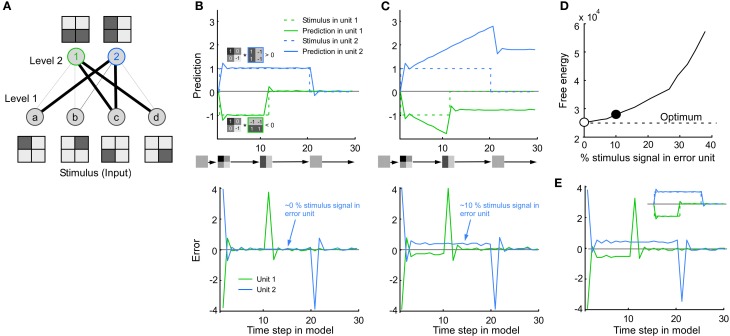
Figure 6.

Consequence of mixing stimulus and error coding in a predictive coding model. (A) The model consists of four input units in level 1 (stimulus pixels) and two output units in level 2 (line detectors), where the line thickness corresponds to the connection weight. (B) Default behavior of the model. Top: Note that the activity in unit 1 and 2 follows the stimulus. The activity in unit 1/2 (green/blue line) is positive/negative since the stimulus image is positively/negatively correlated with the receptive field image of unit 1/2. Bottom: The error is the difference between the stimulus and the activity in the prediction unit. For clarity both prediction and error were taken from the line detectors in level 2, i.e., the error in level 2 was calculated by multiplying the error in level 1 by the connection weights between level 1 and 2. It is important to note that the results also hold for the error units in level 1. (C) To mimic the combination of error and stimulus signal found in this study, the error unit was made to combine stimulus and error signal (bottom). Note that the value of the prediction unit now overshoots the stimulus (top). (D) This divergence from the stimulus can also be quantified in terms of an increase in free energy. Abscissa: 0% means that only the error is represented. This corresponds to the default behavior shown in A (empty circle). Fifty percentage means that the stimulus is represented as much as the error. The example in C has a non-optimal free energy because the model is not made to combine stimulus and error coding (solid circle). (E) By a simple modification of the model the (new) error units can be made to combine stimulus and error at the same time as the prediction unit follows the stimulus (see Inset and Methods).