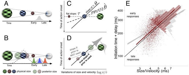
Figure 1. Ambiguity of optical information and predictions.
(A) Inherent ambiguity of monocular optic flow. Three balls (non-transparent) of different sizes (colour for illustrative purposes only) and velocities (blur coded) having the same size to velocity ratio (s/v) will arrive at the point of observation at the same time. The grey histogram reflects a hypothetical distribution of initiation of hand closure responses. (B) Context in which one size is shown more often than others (the medium size blue ball is more frequent and corresponds to the mean of a Gaussian distribution). If a size prior is assumed then the perceived small and large balls (coded as transparent balls) will be biased towards the most probable one (blue one). The distribution of time action initiation for physically deviant sizes (large-green and small-red balls) will be shifted away from that elicited by the mean (blue). (C) Expected distributions of hand closure initiation according to different optical variables when the the time of action (hand closing) onset is plotted against the ratio size to velocity in log-log coordinates. Different slopes denote the use of different variables (see hypothesis testing for details). (D) Example of an expected distribution of initiation times if prior knowledge is used (e.g. the image is assumed to be caused by the most frequent ball). The correct slope will then be observed (i.e. 1/2 and 1 for  and
and  strategies respectively) when the times are plotted against the posterior or perceived size (not the physical ones): the posterior estimate of size
  combines prior information (e.g. transparent balls shifted to the mean). Under this assumption, the model that incorporates the prior, besides yielding the correct slopes, predicts less variability (narrower dark grey Gaussian) and larger systematic error for deviant sizes (small-red and large-green balls). If priors are not used at all, accurate slopes are then again expected when the time distribution is plotted against physical size and velocity (like in panel C). True slopes
  have to be the same when estimated separately on size and velocity (i.e.
  see Eq. 9 for details). (E) Observed distribution of action initiation time as a function of the ratio size to velocity in log-log coordinates for a representative subject.

