
Figure 3.
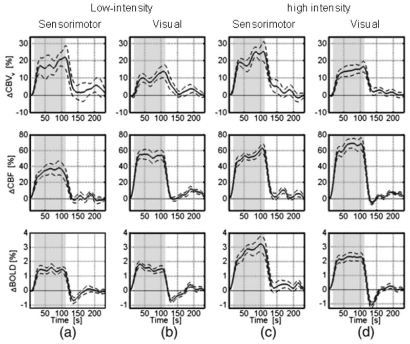
Average time courses for CBVv, CBF and GRE-BOLD obtained during and after 96 s of neuronal activation using (a) low-intensity sensorimotor stimulation (n=11): bilateral tapping at 1.73 Hz; (b) low-intensity visual stimulation (n=13): yellow/blue checker (8 Hz) at 25% contrast; (c) high-intensity (3.46 Hz) sensorimotor stimulation (n=12); (d) high-intensity (8Hz, 100%) visual stimulation (n=14). The dashed lines indicate the standard error, and the stimulation-on period is indicated by the shaded region. Curves are from significantly activated voxels that overlap for all methods, but only the curve with the highest t-value was chosen. In order to enable better visualization of the general transient dynamics, these time courses were smoothed using a low-pass Hanning filter with a 13 s FWHM. Notice the lack of CBF undershoots for sensorimotor and low-intensity visual stimulation as well as fast early CBVv post-stimulus decays followed by very small post-stimulus CBVv variation close to baseline within one standard deviation. Reprinted from Chen and Pike, 2009, Neuroimage. 46, 559, with permission from Elsevier.