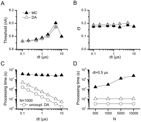
Figure 4. Numerical stability and computational cost of the simulation algorithms with the Rb model. A–B.

Dependence of Rb model variability on the integration time step used in the simulation. Threshold (A) and σ (B) values calculated as in Figure 3A, obtained at different values of integration time step (dt). N = 1000. C. Dependence of computation time on integration time step (dt) with N = 1000 channels. D. Dependence of computation time on number of channels (N) with dt = 0.5 µs. Computation time is the time, in seconds, needed to perform the 16000 simulations necessary for a single firing efficiency curve (1000 pulses at 16 current levels). This figure corresponds to simulations performed in the Scilab numerical computation software. 1000 simulations were performed as 10 batches of 100 simultaneous and independent simulations, in a Core i7 machine. For comparison, the computation time for the uncoupled version of DA is also depicted.