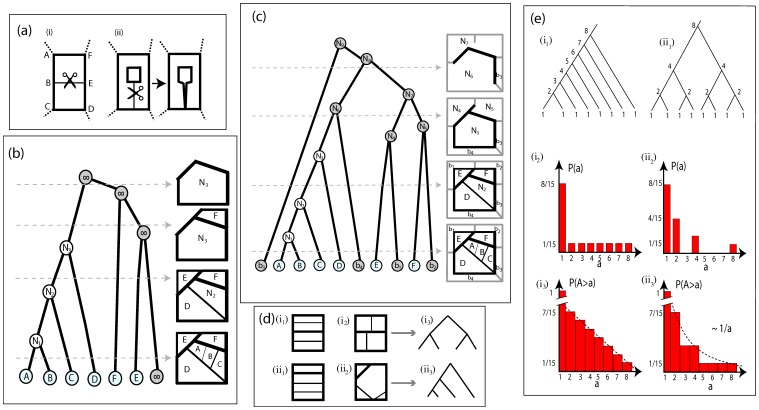
Figure 3. Hierarchical decomposition and nesting trees.

(a) Deletion of an edge in a loopy graph. (i) The deletion of the edge joins two adjacent loops. (ii) The deletion of the edge disconnects the graph. (b) Hierarchical decomposition of a planar graph. Boundary loops sequentially join the outside space, marked as . Left: Nesting tree of the hierarchical decomposition. Right, top to bottom: hierarchically decomposed graph. The bottom right panel corresponds to the full graph, the rest represents the network at different levels of decomposition (the corresponding cutoff level of the tree representation is marked with a gray dashed arrow). As edges of the graph are hierarchically deleted, based on their thickness, the original loops (A–E) are joined to form derived loops (–). (c) Hierarchical decomposition of a planar graph. Phantom boundary loops surround the graph perimeter. Loops contiguous to the perimeter of the graph join a ring of phantom boundary loops. The decomposition proceeds as in (b), but the phantom loops – appear among the loops of the original graph in the tree representation. (d) Building blocks of a loopy architecture. The two basic building blocks of the loopy architecture can be identified using the tree representation of the graph. (i₁),(i₂): multiplicative nestedness. Nested loops merge hierarchically. (i₃): This architecture is represented by “tall” trees. (ii₁),(ii₂): additive nestedness. Ordered loops join consecutively. (ii₃): The tree representation is that of “short” trees. Graphs (i₁) and (i₂) map equivalently to (i₃), similarly graphs (ii₁) and (ii₂) map equivalently to (ii₃). (e) Cumulative size distributions of additive and multiplicative models of nestedness. (i₁) Nesting tree for additive nestedness. The degree of each node is is shown. (i₂) Degree (size) distribution for additive nestedness. (i₃) Cumulatize size distribution for additive nestedness. (ii₁) Nesting tree, (ii₂) Degree (size) distribution and (ii₃) Cumulatize size distribution for multiplicative nestedness.