Protein subcellular location pattern classification in cellular images using latent discriminative models

Abstract

Motivation: Knowledge of the subcellular location of a protein is crucial for understanding its functions. The subcellular pattern of a protein is typically represented as the set of cellular components in which it is located, and an important task is to determine this set from microscope images. In this article, we address this classification problem using confocal immunofluorescence images from the Human Protein Atlas (HPA) project. The HPA contains images of cells stained for many proteins; each is also stained for three reference components, but there are many other components that are invisible. Given one such cell, the task is to classify the pattern type of the stained protein. We first randomly select local image regions within the cells, and then extract various carefully designed features from these regions. This region-based approach enables us to explicitly study the relationship between proteins and different cell components, as well as the interactions between these components. To achieve these two goals, we propose two discriminative models that extend logistic regression with structured latent variables. The first model allows the same protein pattern class to be expressed differently according to the underlying components in different regions. The second model further captures the spatial dependencies between the components within the same cell so that we can better infer these components. To learn these models, we propose a fast approximate algorithm for inference, and then use gradient-based methods to maximize the data likelihood.

Results: In the experiments, we show that the proposed models help improve the classification accuracies on synthetic data and real cellular images. The best overall accuracy we report in this article for classifying 942 proteins into 13 classes of patterns is about 84.6%, which to our knowledge is the best so far. In addition, the dependencies learned are consistent with prior knowledge of cell organization.

Availability: http://murphylab.web.cmu.edu/software/.

Contact: Jeff.Schneider@cs.cmu.edu, murphy@cmu.edu

1 INTRODUCTION

The systematic study of subcellular protein location patterns is required for the full characterization of the human proteome, as these location patterns provide context necessary for understanding the protein's functions. Given Human Protein Atlas (HPA) images that demonstrate the spatial distribution of various proteins and components (organelles) in cells, each of which has been assigned to one of 13 location pattern classes by visual inspection, our goal is to learn to recognize those pattern classes in future images.

We can solve this problem using multiclass classification methods. However, a key difficulty is that we can only observe three types of reference components due to the limitation of staining and imaging techniques. Therefore, it is hard to infer the locations of the invisible components given the observations. For example, we may want to classify a protein into the class of ‘Golgi complex’ if it mainly overlaps with the Golgi complex, but the Golgi complex is not directly visible to us in the images. Thereby, it is important to uncover these invisible parts and then use them for classification from their co-occurrence information with the protein.

Although invisible, we still have some clues about the presence of a component in some region of one cell. For instance, one component may have an effect on the appearance of another overlapping and/or interacting component. We can also make inference about the component in the given image region based on the distribution of certain proteins in the cell (e.g. locations and shapes), and its relative distances to other components. If we can discover the dependencies between the observed features extracted from regions and the underlying components, as well as the co-localization relationships between components, then the presence of those hidden components can be inferred and our classification task would be easier.

We therefore aim at learning from the data the dependencies among features, components and the protein pattern classes into which the images have been divided. To accomplish this, we build two graphical models with latent variables to capture the components and these dependencies. These two models are based on logistic regression (LR) (Bishop, 2006). The first model, called hidden logistic regression (HLR), introduces the concept of component as a latent variable into the simple LR, so that the protein and the component can determine the expressed features together. The second model, called hidden conditional random field (HCRF), further introduces spatial dependencies among components at different locations as in conditional random field (CRF) developed by Lafferty et al., 2001. These two models can capture the components' influence on the expressed features and their spatial configurations, hopefully improving our ability to recognize the patterns.

We use gradient-based methods to estimate the models' parameters. We show that the gradients depend on the marginal probabilities on the nodes and edges in the model. For HLR, this computation is easy. But for the HCRF model, inferences for these marginals cannot be done exactly. To address this difficulty in inference, we propose to remove certain edges in the HCRF model so that the component variables are ‘clustered’. By doing this, the exact inference is greatly accelerated while most of the local interactions between cell components can be retained.

The effectiveness of both the HLR and HCRF models are tested on synthetic data and real HPA images. We show that using latent variables to model the components can enhance the classification accuracy. Furthermore, spatial dependencies can significantly improve the performance. With the proposed models, we are able to achieve the best classification performance on this task to our knowledge.

The rest of the article is organized as below. First, we describe the dataset and define the problem we try to solve in Section 2. Then the proposed classification methods are described in Section 3. Experimental results are shown in Section 4 on both synthetic simulations and real cellular images. In Section 5, we discuss some related work and summarize this article.

2 BACKGROUND

2.1 Dataset

HPA confocal images: the HPA (http://www.proteinatlas.org) is a rich source of location proteomic data (Barbe et al., 2008). It contains confocal immunofluorescence images for multiple cell lines stained for thousands of proteins with multiple reference channels. Standard stains for the nucleus, endoplasmic reticulum (ER) and cytoskeleton are imaged. In addition, one particular protein is stained in each image, using a monospecific antiserum. Hence each image of a cell includes four fluorescence channels. One example of such image is shown in Figure 1. The images are visually annotated with a class label for the subcellular location of the protein. For the experiments in this article, we chose a subset of the HPA images consisting of 1882 images of 942 proteins from one of 13 classes: centrosome, cytoplasm, actin filaments, intermediate filaments, microtubules, ER, Golgi, mitochondria, nuclei, nucleus without nucleoli, nucleoli, plasma membrane and vesicles.

Fig. 1.

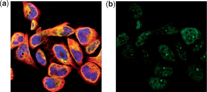
One sample image from the HPA data set. The (a) shows the three reference channels reflecting different components (blue:nucleus, yellow:ER and red:cytoskeleton). The (b) shows the channel of the stained protein (green)

To preprocess the image data, we first used the seeded watershed method to segment the image fields into single cells (Newberg et al., 2009). After that, for every cell we randomly select 50 regions of size 41×41 pixels, each of which must contain some of the stained protein signal (i.e. not empty). The size is chosen so that an individual region captures fine enough information about the specific component in it, and the number of regions is chosen so that most of the area of the cell is covered while it is computationally feasible to solve the problem.

To extract features from the sampled regions, we compute various subcellular location features according to Newberg et al., 2009 on individual channels separately as well as on the combinations of different channels. These features essentially characterize the appearance, the texture information, the multi-resolution aspect and the spatial distribution of different cell components in the image regions. After feature extraction and removing bad regions and cells, we have 15 990 cells, containing 799 015 regions with 2538 dimensional features.

2.2 Problem definition

To begin with, we give a brief re-statement of the problem. The data we have is a set of cellular images. For each small rectangular region in those images, we can observe some vector of features, and we know the class of the protein stained in this cell and region. Given these data, our goal is to train a model that can classify the distribution pattern of the protein stained in unlabeled images.

We introduce some notations here. Suppose there are N cells containing M image regions, T types of cell components and K classes. The features we have for region m is F_m∈ℝ^D_F, where D_F stands for the size of feature. For this region, we have a label C_m indicating the class of the stained protein.

3 PROPOSED METHODS

3.1 The Latent Discriminative Models

We take a discriminative approach and design models to solve the classification problem directly.

The most straightforward way of modeling is to let the region's protein class label C_m directly determine the features F_m we observe in that region. We can describe this simple model using the undirected graphical model in Figure 2.

Fig. 2.

The LR model for regions. F_m are the features and C_m is the label

We adopt a discriminative approach here. Instead of modeling the joint probability of the labels and features, we directly characterize the probabilities of labels conditioned on the features, since our focus here is prediction. Based on this principle, we can use a log-linear model to realize the model in Figure 2 as follows:

(1)

where the parameter set Θ contains w₁,···, w_K, one for each class, and the footnote T in all equations stands for transpose. We can see that this model is in fact LR for multi class problems. After training, the LR model is able to predict the class label for each test region, based on which cell- and protein-level predictions can be obtained by voting. This simple LR model is our starting point.

3.1.1 HLR

The LR model implies the assumption that the region features F_m are solely determined by the protein label C_m in that region. This assumption is obviously inadequate in our problem. Clearly, the features (appearance) of a region are determined by both the protein and the cell component(s) in it. Therefore, in addition to the protein variable C_m, we introduce a new variable O_m to represent the component(s) in that region, and let C_m and O_m determine the features F_m together.

The resulting graphical model is shown in Figure 3. Note that we only have the cellular images and do not know the value of O_m for each region. So, O_m is a latent variable and has to be inferred.

Fig. 3.

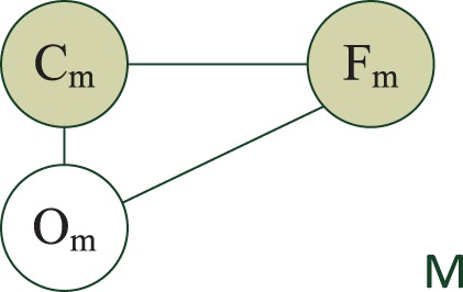
The HLR model for regions. O_m is the latent variable categorizing the underlying cell component(s)

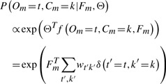
We again use a log-linear model to characterize what is in Figure 3. The conditional probability of the protein label C_m and the component O_m can be written as:

(2)

where Θ are the linear parameters, f(·) is a class-dependent feature function and the last line shows the concrete form of this conditional probability. Intuitively, this model is an extended multiclass LR model in which we treat each pair of (O_m, C_m) as one class, and then normalize the probability globally. We refer to it as the HLR model.

While the conditional probability above is intuitive, we cannot directly maximize the likelihood under this model, since the values of {O_m} are not observed. Therefore, we instead estimate the parameters by maximizing the marginal probability of the labels as below:

(3)

The results produced by HLR are still region-level classification. In the following, we consider the structural information within the cell.

3.1.2 HCRF:

in the HLR model, we relax the assumption that the features of different regions are identically distributed given the protein class label, and let one protein class be expressed differently at different parts of the cell. But we are still assuming that the regions are independent of each other. However, in fact, we know that there are spatial dependencies among the components. For example, the Golgi complex is usually located near the nucleus. So when we see the nucleus, which is easy to recognize, we have some clue that the Golgi complex will be nearby. This type of reasoning is frequently used when human experts try to classify a protein pattern. Our next step is trying to emulate this process and capture the spatial dependencies among the components.

Unlike previous sections where we focus on regions, here we treat cells as the units in classification. For cell n, we let M_n be the number of regions in it. Further, F_n/G_n, C_n are the features and the label for the cell n, and O_n,m is the component(s) in the m-th region of the cell n.

The new model extends HLR described in Section 3.1.1 by allowing the components in the same cell to interact with each other. The graphical model that captures all the dependencies is shown in Figure 4.

Fig. 4.

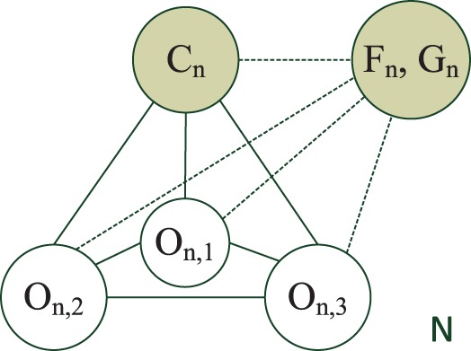
The HCRF model for cells. All the components {O_n,m} are latent variables

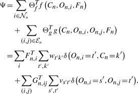
As before, we use log-linear models to characterize the dependencies between variables, as in CRF by Lafferty et al., 2001. The conditional probability of the protein label and component is as follows:

(4)

(5)

where , are the node and edge sets. In this model, the parameter set Θ includes {w_tk} and {v_st}. The association features F_n,i∈ℝ^D_F provide evidence for an individual region i, and the interaction feature G_n,ij∈ℝ^D_G provides evidence for the dependency between a region pair (i, j). {w_tk} define the potential on each region and {v_st} define the potential for pairs of regions. As before, the components O_n are not observed. We call this model the HCRF.

To learn this model, we also need to maximize the marginal likelihood of the labels C_n. That is, our goal is to solve the problem in the following:

(6)

Note that unlike LR and HLR, HCRF is able to produce cell-level prediction directly.

3.2 Learning

In this section, we describe how to learn the proposed HLR and HCRF models, and use them for prediction.

3.2.1 Training

We use gradient-based optimization to train the parameters of the HLR and HCRF models. As shown in Section 3.1, the goal of learning is to maximize the marginal probability of the data:

(7)

In log-linear models, the conditional probabilities in general can be written as:

(8)

Meanwhile, the marginal of the label C_n can be written as follows:

(9)

(10)

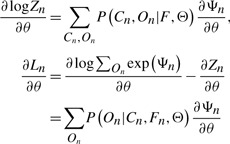
By taking the derivative of L_n with respect to some parameter θ, the following results can be derived:

(11)

(12)

(13)

From Equation (13), it is easy to obtain the derivative for any parameter in HLR and HCRF. Here, we omit the details and only show the final results.

For the HLR model, the derivatives are

(14)

For the HCRF model, the derivatives are

(15)

(16)

Given these results, we can use gradient-based optimizers to train the parameters by maximizing the marginal likelihood of the data. For example, we can use L-BFGS (Nocedal and Wright, 2000) or stochastic gradient descent (Bottou, 1998). Note that the key quantities required to calculate these gradients are the marginal probabilities in the forms of P(O|C, F) and P(C, O|F).

3.2.2 Inference

In Section 3.2.1, we have derived that in order to apply gradient-based learning, we need to first calculate the marginal probabilities in the forms of P(O|C, F) and P(C, O|F). Therefore, inference algorithms are necessary.

For the HLR model, inference is straightforward since the number of terms in the partition function is only T×K. We can easily enumerate all of them to get the exact values of those marginal probabilities. Given the exact gradients and the objective values, we apply L-BFGS to learn the HLR model.

For the HCRF model, the inference problem becomes intractable because of the dependence structure of the graphical model. Brute force is infeasible since the partition function contains K×T^M terms, where M is the number of regions in one cell. Other exact methods such as variable elimination (Koller and Friedman, 2009) are also not viable because the nodes can be densely connected and therefore the tree width (Koller and Friedman, 2009) of the graph, which determines the complexity of inference, can be very large. Therefore, we need approximate methods.

Unfortunately, classical approximate inference methods are difficult to apply here. For example, mean field approximation (Koller and Friedman, 2009) is not applicable because we need the marginal probabilities on edges, which are not available from a completely factorized mean field distribution. The choice of belief propagation (BP) (Pearl, 1988) seems reasonable considering the forms of derivatives in Equation (15) because it provides all the marginal probabilities we need. However, the HCRF model contains numerous small loops like ‘C-O-O’ and ‘O-O-O’ in Figure 4, which make the BP algorithm inaccurate or even non-convergent. Moreover, the approximate inference result will prevent the marginal likelihood from being optimized efficiently, due to the fact that we cannot evaluate the objective value correctly.

To solve these problems, we propose to use an approximate model and exact inference, as opposed to using an exact model and approximate inference. Concretely, we first reduce the tree width of the model and then use variable elimination for inference. We partition the latent ‘O’ nodes of HCRF into small clusters, then the tree width is equal to the largest cluster size. For example, given that a cell contains 50 components in regions, we can partition these components into 10 clusters of size 5 based on their spatial locations in the cell. Then, we remove the ‘O-O’ edges that cross cluster boundaries, while still keeping all the ‘C-O’ edges. By doing this, the tree width of the model is always limited to a small number regardless of the total number of components (regions), making exact inference by variable elimination tractable.

An illustration of this process is shown in Figure 5. We can see that by making this simplification of model, we lose a few edges, but most of the important local interactions between regions are kept. In return, the inference and learning of the simplified model become efficient. Suppose there are M regions in one cell and we partition them into clusters of size s. Then after the partition, inference can be done in O((M/s)KT^s). Note that now the complexity grows only linearly with the number of regions. However, it still grows exponentially with the cluster size s, which therefore cannot be large. Note that when s=1, the HCRF degenerates into HLR.

Fig. 5.

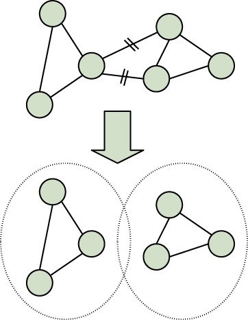
An illustration of how to simply HCRF for tractable exact inference. Each node represents an ‘O’ node in HCRF

3.2.3 Implementation

To construct the interaction graphs of HCRF among the components within the same cell, we add edges between components and their nearest neighbors. In this article, we always use the three nearest neighbors to build the interaction graph. Currently, the feature G on each edge in HCRF is just the distance between the centers of two regions. In the future, we may add more descriptive features for the edges.

Since we have adopted the ‘approximate model, exact inference’ approach, both the gradient and the objective value of the data likelihood can be computed exactly, making the optimization straightforward. Here, we use L-BFGS to maximize the marginal likelihood due to its fast convergence and low-memory consumption.

It should be pointed out that HCRF has a large number of parameters. In order to avoid overfitting and enhance the generalization ability, we regularize the L₂-norm of the parameters as in ridge regression with a penalization parameter λ. This part is straightforward and details are omitted.

Since the time required to infer the HCRF model grows exponentially with the cluster size into which regions are grouped, we set the cluster size to 5 with tradeoff between speed and approximation accuracy. With this setting and T=3, inference took ~20 h on one 2.40 GHz 64-bit processor for the HCRF model. The HLR model took about 10 min when T=3.

4 EXPERIMENTS

In this section, we show the performance of the proposed methods on both synthetic data and real HPA images.

4.1 Simulation

First, we ran a simulation experiment to verify the effectiveness of latent variables in HLR and HCRF. The synthetic data contains M=10 000 regions, D=10 dimensional feature vectors, T=3 types of components and K=3 classes of protein. To generate such a data set, we use the mechanism described in Figure 3. This experiment aims at showing that ordinary LR is not able to handle the case where features depend on factors other than just the label.

The HLR model is used here. We try T from 1 to 10 and compare the performance. For every T, we run 10 times of 5-fold cross-validations. Due to the non-convexity of the HLR model, in each training step of each run, we try five random starts, and pick out the one with the maximum training accuracy. The best value of λ is picked from 0.01 to 1000 also using cross-validation.

The mean accuracies for different values of T are shown in Figure 6. Standard deviations are not shown since they are very small. We can see that when the number of latent components are less than the true value T=3, the performance is poor. Once we use T≥3 components, nearly perfect accuracies have been achieved. Note that from Equation 2 when T=1, the HLR model is equivalent to the regular multiclass LR. Moreover, note that for T≥3, little sign of over-fitting is observed. The results demonstrate that incorporating latent components for this problem greatly helps.

Fig. 6.

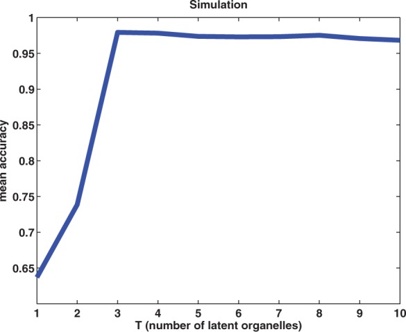
Results of the simulation study, showing the accuracies of various choices of T (the number of latent components). The true number of components is T=3

4.2 HPA protein classification

We also compare the performance of different methods on the HPA data set. As described before, we have M=799 015 regions, D_F=2538 dimensional features for each region and K=13 protein pattern classes. These regions are from 15990 cells and 942 proteins. After applying PCA to reduce the feature dimension, we obtained D_F=131 features for each region. This data set suffers from moderately imbalanced class distribution problem, in which ~30% of the samples belong to the largest class.

The Support Vector Machine (SVM) is used as our baseline. We use linear SVM [liblinear 1.5.1 (Fan et al., 2008)] to classify these regions. We predict the labels and the class probabilities for regions in 5-fold cross-validations and automatic tuning of the slack parameter C. Then we let the region results vote for the cell-level labels as follows. For each cell, we add together the class probabilities of all the regions from this cell, and then normalize the sum as the class probabilities for this cell. The class with the maximum probability is selected as the label for this cell. Using the same voting schema, we can also obtain labels and the associated probabilities for the proteins.

After using five different runs of cross-validation with random partitioning, we obtain that the resulting overall accuracies for proteins are 69.1 ± 0.25%. In addition, for the best run, we plot the precision and recall curve in Figure 8 using the following procedure. We first sort the proteins by the magnitude of the maximum probability value (voted from the cells as above) for each protein. An increasing threshold on this probability is used to generate this precision-recall (PR) curve. The precision is calculated as the number correct divided by the number of proteins classified with probability above the threshold. The recall is defined as the number correct divided by the total number of proteins. The area under the curve (AUC) is 0.60. It is important to note that in this and all experiments in this article, when we split the data set into training and testing sets for cross-validation, all of the regions and cells belonging to the same protein were in either the training or the testing set (i.e. the same protein cannot be in both the training the testing sets simultaneously). As a result, the learner must generalize across different proteins with the same label and the accuracy might be conservative.

Fig. 8.

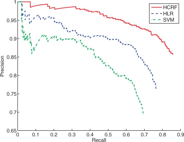
Precision and recall curves on protein classification probabilities from SVM, HLR and HCRF. Each of them is from the one having the best overall accuracy

We first test the performance of the HLR model on this dataset. We use T from 1 to 10, and other settings are similar to those in Section 4.1 and in the SVM experiment. The mean performance and standard deviations for the voted accuracies on proteins are shown in Figure 7. A clear improvement is achieved when increasing T from 1 to 2. The highest mean accuracy is ~80.7%, achieved when T=2. For the best run of cross-validation in T=2, a PR curve is plotted in Figure 8 and the AUC is 0.69. Therefore, HLR outperforms the basic LR (the T=1 case) and the SVM baseline significantly. This result again verifies the effectiveness of the latent components.

Fig. 7.

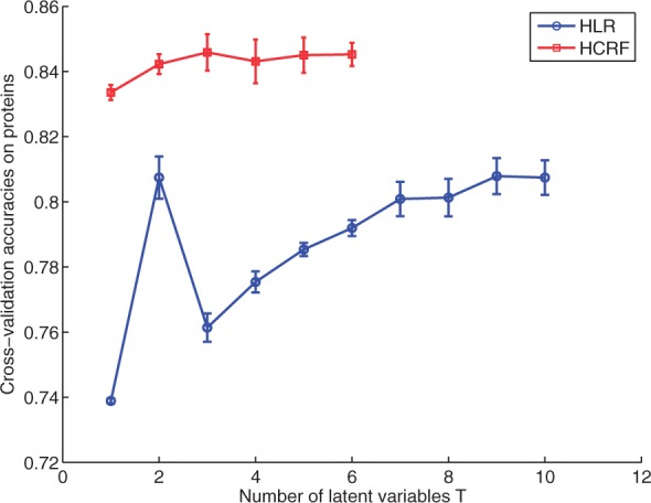
Classification accuracies on HPA proteins by HLR and HCRF. These accuracies are obtained from cell-level results by probability voting

Next, we test the performance of HCRF in the task of classifying the cells and proteins. In this case, we can only afford the time and memory usage to try T from 1 to 6. For efficient inference, we divide the regions in each cell into clusters of size 5 as described in Sections 3.2.2 and 3.2.3. We do five runs on each T to get the mean and variance of the performance. In each run, we use a different seed to randomly split the data and do 5-fold cross-validation. Again at the beginning of every training step, we use five trials of random starts and the one with the maximum training accuracy will be used to do the testing.

The resulting accuracies are shown in Figure 7. We can see that the HCRF model significantly improves the accuracies over the HLR model. The best mean overall accuracy on the protein level that is obtained by voting across cells is 84.6% acquired when T=3, and the confusion matrix for best run with T=3 is shown in Table 1. The confusion matrix shows that larger classes tend to have higher accuracies. The nuclei pattern is often confused with the ‘nucleus without nucleoli’ pattern because the latter has many more member proteins and these are often difficult to distinguish visually. This is also the case for proteins of the plasma membrane and cytoplasm classes. For the best cross-validation run, we plot the PR curve in Figure 8, which has an AUC of 0.82. From the figure, we can see that if we increase the threshold to have recall of ~60%, the precision is ~95%.

Table 1.

Confusion matrix of classification on proteins using HCRF model

Accuracy%	centro.	cyto.	actin	inter.	micro.	er	golgi	mitoch.	nuclei	w/o	nucleoli	PM	vesicle
Centrosome (15)	40	6.7	0	0	0	0	20	0	0	13.3	0	0	20
Cytoplasm (125)	0	92	0	0	0	0	0	3.2	0	0	0	0.8	4
Actin filaments (10)	0	20	10	0	0	0	0	30	0	10	0	10	20
Intermediate filaments (12)	0	8.3	0	66.7	0	0	0	25	0	0	0	0	0
Microtubules (18)	0	5.6	0	0	94.4	0	0	0	0	0	0	0	0
ER (39)	0	0	0	0	0	89.7	0	7.7	2.6	0	0	0	0
Golgi (63)	0	1.6	1.6	0	0	0	81	9.5	1.6	0	0	1.6	3.2
Mitochondria (148)	0	0.7	0	0	0	0	0	99.3	0	0	0	0	0
Nuclei (75)	0	0	0	0	0	0	0	0	37.3	57.3	5.3	0	0
Nucleus w/o nucleoli (284)	0	0	0	0	0	0	0	0	1.4	96.8	1.8	0	0
Nucleoli (65)	0	1.5	0	0	0	0	1.5	0	3.1	4.6	87.7	0	1.5
Plasma membrane (14)	0	35.7	21.4	0	0	0	7.1	7.1	0	7.1	0	14.3	7.1
Vesicles (74)	0	1.4	1.4	0	0	0	4.1	2.7	1.4	1.4	0	0	87.8

It is the one having best overall accuracy from trails of T=3. The values in the parentheses are the numbers of proteins in each class.

Since the HCRF with T≥2 outperforms the one with T=1, we can conclude that the latent components and spatial dependencies introduced in HCRF are indeed useful.

Note that the overall accuracy appears to saturate at around 84 in Figure 7. We have estimated that the overall accuracy of human annotation of these labels in other work is ~90% (data not shown), which our classification accuracy approaches. Moreover, any errors in labeling by human experts may result in confusion when used for training the classifiers. Therefore, we believe that the accuracy achieved by HCRF is indeed approaching the limit, although there is probably some room for improvement.

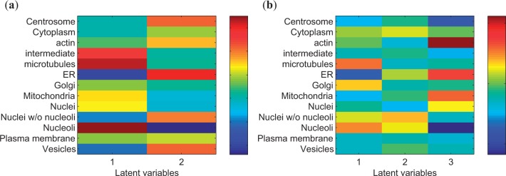
To provide further insight into the basis for the improvement in accuracy by HLR or HCRF, we investigate the meaning of the latent components learned from data and their relationships with the classes of protein distribution patterns. To interpret these components, we infer the matrix P(C_m, O_m|F_m, Θ) of size of K×T using Equations (2) and (14), or (15) for each region. The calculation is based on the setting that produces the best overall accuracy. We then sum the matrices over all the regions to get one matrix that represents the co-occurrence relationship between C and O. After being normalized so that the entries sum to one, this matrix can represent the co-occurrence probabilities between the classes and latent components. We show the probability maps from HLR and HCRF in Figure 9.

Fig. 9.

Two probability maps representing the co-occurrence relationships between the learned latent components and classes. (a) is from HLR and (b) is from HCRF

From Figure 9, we can see the distinct relationships between different latent components and different classes. Each latent component is associated with a unique combination of classes. In Figure 9 (a), the two latent components mostly differ in the distribution relative to nucleus, i.e. close to nucleus (the first) or not (the second). The first one has larger coefficients on intermediate filaments and microtubules, because the projection from 3D distribution onto the 2D image makes these two have high intensity within and around the nucleus area. The ‘Nuclei’ pattern and ‘Nuclei without nucleoli’ pattern are distinct, so they should be in different components. This also explains the phenomenon in Figure 7 that HLR apparently do better with two components than with ≥3 components, because HLR may find the most conspicuous clue for identifying the location patterns of proteins to be inside or near to the nucleus or outside. Other clues compared to the nucleus may have little help or even hurt by overfitting (actually the training likelihood still grows as T increases, data not shown). In Figure 9 (b), the first latent component again represents the patterns distributing inside or tightly close to nucleus, the second involves granular distribution over the cytosolic space and the third involves smooth distribution over the cellular space (including the nucleus).

5 DISCUSSION

5.1 Related work

Recently, there have been several studies using latent discriminative models to solve structured prediction problems with partially observed data. Here, we discuss the most relevant two. Our proposed HCRF model is similar to the work Discriminative Random Field by Kumar and Hebert, 2004. The difference is that in our case the labels for the regions are latent variables, and each cell has only one label. The concept of HCRF has also been raised in the work done in Quattoni et al., 2007, and the structure of their graphical model is quite similar to ours; nevertheless, in their model, the cell label is only associated with the latent labels of the regions. In our model, these connections are also conditioned on the observations, which reflects the fact that the protein classes and the latent components determines the features together.

The only prior work on the automated classification of proteins using HPA immunofluorescence images is by Newberg et al., 2009. In that article, each cell is treated as a single region, and SVM directly applied to classification. The experiment using that approach on the dataset used here gives the overall accuracy on proteins to be 81.3%±0.61%. Therefore, our HCRF model is statistically better.

5.2 Conclusion

In this article, we address the problem of classifying proteins based on their subcellular localization patterns. Given the spatial distribution of a protein in the cells, we want to know the class of this protein.

To solve this problem, we proposed two discriminative models that extend LR with latent variables. The first one, called the HLR, extends regular logistic regression so that the features can depend on factors other than the class label. The HLR model addresses the issue that the same protein can be expressed differently at different locations of the cell. The second model, called the HCRF, further extends the HLR model by allowing the regions in the same cell to interact with each other. HCRF is able to ‘guess’ the component at a location based on information from other regions, thus helping us better predict the class of the protein.

In both synthetic and real data experiments, we demonstrate that the proposed models are able to enhance classification performance. Particularly, on the HPA dataset, HCRF achieved 84.6% overall accuracy on proteins, which is best result up to now.

In the future, we plan to enhance the performance by using better features and devise more accurate learning algorithms. For example, we can incorporate richer dependencies between components. The features can also be transformed to take potential non-linearity into considerable. More efficient inference algorithm can be developed to allow for more complex interactions between components. Moreover, because there are much larger amounts of images of proteins that can localize in more than one component in cell, we want to apply the models proposed in this article to classify more challenging protein subcellular location pattern complexes.

REFERENCES

- Barbe L., et al. Toward a confocal subcellular atlas of the human proteome. Mol. Cell Proteomics. 2008;7:499–508. doi: 10.1074/mcp.M700325-MCP200. [DOI] [PubMed] [Google Scholar]
- Bishop C.M. Pattern Recognition and Machine Learning. Springer; 2006. pp. 203–213. [Google Scholar]
- Bottou L. Online algorithms and stochastic approximations. In: Saad D., editor. Online Learning and Neural Networks. Cambridge, UK: Cambridge University Press; 1998. [Google Scholar]
- Fan R., et al. Liblinear: a library for large linear classification. The Journal of Machine Learning Research. 2008;9:1871–1874. [Google Scholar]
- Koller D., Friedman N. Probabilistic Graphical Models: Principles and Techniques. The MIT Press; 2009. pp. 285–486. [Google Scholar]
- Kumar S., Hebert M. Discriminative fields for modeling spatial dependencies in natural images. In: Thrun S., et al., editors. Advances in Neural Information Processing Systems 16. The MIT Press; 2004. pp. 1531–1538. [Google Scholar]
- Lafferty J., et al. Conditional random fields: Probabilistic models for segmenting and labeling sequence data. In: Brodley C.E., Danyluk A.P., editors. 18th International Conference on Machine Learning. Morgan Kaufmann; 2001. pp. 282–289. [Google Scholar]
- Newberg J.Y., et al. Proceedings of the 2009 IEEE International Symposium on Biomedical Imaging: From Nano to Macro (ISBI 2009). IEEE Press; 2009. Automated analysis of human protein atlas immunofluorescence images; pp. 1023–1026. [DOI] [PMC free article] [PubMed] [Google Scholar]
- Nocedal J., Wright S. Numerical Optimization. Springer; 2000. pp. 222–248. [Google Scholar]
- Pearl J. Probabilistic Reasoning in Intelligent Systems: Networks of Plausible Inference. Morgan Kaufmann; 1988. pp. 143–236. [Google Scholar]
- Quattoni A., et al. Hidden conditional random fields. IEEE Trans. PAMI. 2007;29:1848–1853. doi: 10.1109/TPAMI.2007.1124. [DOI] [PubMed] [Google Scholar]