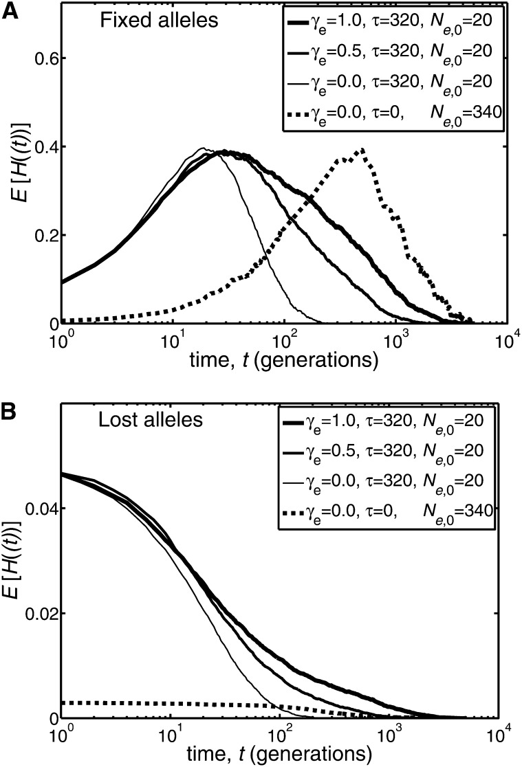
Figure 2 .
Illustration of the behavior of the mean heterozygosity E[H(t)] [where H(t) = 2X(t)(1−X(t))] as a function of the time, t, when the effective population size has a period of linear growth, as in Equation 15. The results presented were derived from simulations of 2 × 10⁴ replicate populations, which were run until either fixation or loss occurred. Binomial sampling was used, and hence actual and effective population sizes coincided. A single copy of a mutant allele was assumed present at time t = 0. The heterozygosities plotted are conditional on the mutant alleles either fixing (A) or being lost (B). The solid lines correspond to an initial effective population size of Ne,0 = 20 and a duration of linear growth of τ = 16 × Ne,0 = 320 generations. For comparison, the dashed line corresponds to a population of constant effective size, whose value is the largest size achieved by a population with γe = 1 and Ne,0 = 20; namely, Ne,0 = 20 + 320 = 340.

