Joint L¹ and Total Variation Regularization for Fluorescence Molecular Tomography

Abstract

Fluorescence molecular tomography (FMT) is an imaging modality that exploits the specificity of fluorescent biomarkers to enable 3D visualization of molecular targets and pathways in vivo in small animals. Owing to the high degree of absorption and scattering of light through tissue, the FMT inverse problem is inherently illconditioned making image reconstruction highly susceptible to the effects of noise and numerical errors. Appropriate priors or penalties are needed to facilitate reconstruction and to restrict the search space to a specific solution set. Typically, fluorescent probes are locally concentrated within specific areas of interest (e.g., inside tumors). The commonly used L² norm penalty generates the minimum energy solution, which tends to be spread out in space. Instead, we present here an approach involving a combination of the L¹ and total variation norm penalties, the former to suppress spurious background signals and enforce sparsity and the latter to preserve local smoothness and piecewise constancy in the reconstructed images. We have developed a surrogate-based optimization method for minimizing the joint penalties. The method was validated using both simulated and experimental data obtained from a mouse-shaped phantom mimicking tissue optical properties and containing two embedded fluorescent sources. Fluorescence data was collected using a 3D FMT setup that uses an EMCCD camera for image acquisition and a conical mirror for full-surface viewing. A range of performance metrics were utilized to evaluate our simulation results and to compare our method with the L¹, L², and total variation norm penalty based approaches. The experimental results were assessed using Dice similarity coefficients computed after co-registration with a CT image of the phantom.

1. Introduction

Inverse operators for ill-posed (or ill-conditioned) problems tend to be unbounded (or have a very large norm). Regularization is the use of bounded (or low-norm) approximations for such inverse operators that allow us to generate meaningful and numerically stable solutions (Daubechies et al. 2004). This typically involves incorporating some prior knowledge usually in the form of a penalty function that controls some desired property of an unknown deterministic variable or the prior probability distribution of an unknown random variable. In the context of image reconstruction, for example, penalty functions are often chosen to enforce smoothness (Fessler and Hero 1995), preserve edges (Lange 1990,Strong and Chan 2003), promote sparsity (Mohajerani et al. 2007, Cao et al. 2007, Gao and Zhao 2010a), or incorporate anatomical information (Leahyand Yan 1991, Fessler et al. 1992, Hyde et al. 2010).

The most widespread method for handling the ill-conditioning of inverse problems is Tikhonov regularization (Tikhonov and Arsenin 1977), in which the cost function contains an L² norm penalty term in addition to the data-fitting term. For the linear system Ax = b, with system matrix A, unknown vector x, and data vector b, the Tikhonov regularized solution is the minimizer of the cost function:

$$\Phi \left(\mathit{\text{x}}\right)=\frac{1}{2}{\Vert \mathit{\text{Ax}}-\mathit{\text{b}}\Vert }_2^2+\frac{\lambda }{2}{\Vert \Gamma \mathit{\text{x}}\Vert }_2^2,$$ (1)

where Γ is an appropriately chosen Tikhonov matrix. In the simplest case, in which Γ = I, this regularization technique favors solutions with lower L² norms. The Bayesian implication of Tikhonov regularization is the assumption of a multivariate Gaussian probability distribution on the unknown random vector.

The goal of fluorescence molecular tomography (FMT) is to compute the 3D distribution of a fluorescent source inside a volume from the photon density detected on the surface (Dutta et al. 2008, Weissleder and Ntziachristos 2003, Eppstein et al. 2002). The fluorescent source may be a near infrared (NIR) fluorescent dye, an active or activatable fluorescent biomarker, or a fluorescent protein expressed by a reporter gene (Shu et al. 2009, Massoud and Gambhir 2003). FMT is a promising low-cost molecular imaging modality that does not use any ionizing radiation and exploits the availability of a variety of highly specific fluorescent molecular markers. Yet, this technique is confounded by the high degree of absorption and scattering of photons propagating through tissue, making the FMT problem ill-conditioned. Approaches for alleviating this problem and improving source localization include multispectral illumination and/or detection (which exploit the spectral variation of tissue optical properties) (Gardner et al. 2010, Li et al. 2009, Chaudhari et al. 2009, Zacharakis et al. 2005) and the use of multiple spatial patterns of illumination (Dutta et al. 2010, Bélanger et al. 2010, Dutta et al. 2009, Joshi et al. 2006) to increase the information content in the collected data. While these approaches improve the conditioning of the FMT system matrix, image reconstruction continues to be highly susceptible to the effects of noise and numerical errors, necessitating the use of some kind of regularization.

While the simple Tikhonov regularizer generates moderately satisfactory results when applied to FMT reconstruction, we would like to design an improved regularizer that specifically takes into account prior knowledge about FMT images. A variety of regularizers have been reported in the fields of FMT, diffuse optical tomography, and bioluminescence tomography (Hyde et al. 2010, Pogue et al. 1999, Axelsson et al. 2007, Li, Boverman, Zhang, Brooks, Miller, Kilmer, Zhang, Hillman & Boas 2005, Guven et al. 2005). We focus on the fact that NIR probes used in FMT are designed to preferentially accumulate in specific areas of interest, e.g., tumors or cancerous tissue. Therefore, reconstructed FMT images commonly exhibit fluorophore concentrations localized within tumors and the major excretory organs (Bloch et al. 2005, Weissleder et al. 1999). Consequently these images tend to be very sparse with some locally smooth high intensity regions. This inspires us to investigate a combination of regularizers that enforce conditions of sparsity and smoothness on reconstructed FMT images.

The most fundamental sparsity metric is the L⁰ norm, which isthe total number of non-zero elements in a vector. However, the L⁰ norm-penalized inverse problem, at least in the underdetermined case, is NP-hard (Natarajan 1995). Instead, the L¹ norm, which is a convex relaxation of the L⁰ norm,is often used to enforce sparsity in images and is particularly popular in the field of compressed sensing (Donoho 2006, Candes and Wakin 2008). The corresponding optimization problem can beformulated in a number of equivalent ways including basis pursuit, where the L¹ norm appears in the cost function and the L² data-fitting term appears in the constraint (Chen et al. 1998), least absolute shrinkage and selection operator (commonly referred to as LASSO), where the L² data-fitting term appears in the cost function and the L¹ norm appears in the constraint (Tibshirani 1996), and L¹-penalized least squares, where the L¹ norm penalty weighed by a regularization parameter is added to the L² data-fitting term to construct the cost function. Approaches to solve these problems include pivoting algorithms (Efron et al. 2004), interior-point methods (Kim et al. 2007), and gradient-based techniques (Daubechies et al. 2004, Figueiredo et al. 2007, Beck and Teboulle 2009). In this work, we choose the L¹ penalty for enforcing sparsity in FMT images.

A variety of smoothing priors have been applied to tomographic reconstruction (Hebert and Leahy 1989, Green1990). Amongst these, priors involving quadratic penalties are particularly common, since they are easy to handle. However, they tend to smooth out edges in images. We, therefore, choose to use the total variation (TV) penalty, which promotes smoothness while preserving edges in images (Rudin et al. 1992). Inthis work, we define the total variation as the L¹ norm of the differences between neighboring pixels. This particular form of the TV penalty enforces sparsity on pixel differences and consequently tends to generate images with piecewise constant regions and sharp boundaries. A variety of methods have been employed for handling the TV penalty, including dual-based and interior point approaches (Chambolle 2004, Vogel and Oman 1998, Huang et al. 2008, Gao and Zhao 2010b). In this work, we derive a method based on the separable paraboloidal surrogates (SPS) algorithm for minimizing the TV penalty.

Section 2 describes a compound approach that uses a combination of the SPS method with the preconditioned conjugate gradient (PCG) algorithm for handling the joint L¹ and TV penalties. We use ordered subsets to accelerate the SPS approach. In section 3, we describe an experimental setup based on a mouse-shaped phantom for testing the joint penalties. We validate our method by applying it to both simulated and experimental data. A discussion and analysis of our simulation and experimental results is presented in section 4.

2. Methods

The cost function we seek to minimize contains three parts – a data-fitting term, a sparsifying penalty term, and a smoothing penalty term. As mentioned before, the sparsifying penalty under consideration is the L¹ norm of the unknown image x. For smoothing the 3D image x, we penalize its total variation, defined as follows:

$$\mathit{\text{TV}}\left(\mathit{\text{x}}\right)=\sum _k|{\mathit{\text{x}}}_{m\left(k\right)}-{\mathit{\text{x}}}_{n\left(k\right)}|,$$ (2)

where m(k) and n(k) are pixel indices corresponding to the kth neighboring pixel pair in the 3D image x. The resulting optimization problem is as follows:

$$\widehat{\mathit{\text{x}}}=\text{arg}\underset{\mathit{\text{x}}\ge 0}{\text{min}}\frac{1}{2}{\Vert \mathit{\text{Ax}}-\mathit{\text{b}}\Vert }_2^2+{\lambda }_{L^1}{\Vert \mathit{\text{x}}\Vert }_1+{\lambda }_{\mathit{\text{TV}}}\sum _k\left|{\mathit{\text{x}}}_{m\left(k\right)}-{\mathit{\text{x}}}_{n\left(k\right)}\right|.$$ (3)

Here λ_L1 and λ_TV are regularization parameters.

In FMT, the non-negativity constraint on the unknown vector helps us circumvent any complications due to the non-differentiability of the L¹ norm penalty near zero. Let us consider two functions f₁(x) = g(x) + ‖x‖₁ and f₂(x) = g(x) + x. Then, min_x≥0 f₁(x) = min_x≥0 f₂(x). This allows us to simplify the L¹ norm penalty to a linear term. To handle the non-differentiability of the TV penalty, we approximate it as follows:

$$\mathit{\text{TV}}\left(\mathit{\text{x}}\right)\approx {\Phi }^{\mathit{\text{TV}}}\left(\mathit{\text{x}}\right)\triangleq \sum _k\sqrt{{\left[\mathit{\text{Cx}}\right]}_k^2+{\delta }_{\mathit{\text{TV}}}},$$ (4)

where the transformation υ = Cx computes nearest neighbor differences and C ∈ ^nn×n_s, n_s being the number of pixelsin x and n_n being the number of neighboring pixel pairs. The parameter δ_TV tends to round off sharp edges when large but leads to instability as it approaches machine precision (Vogel and Oman 1996, Chan et al. 1996). We set it to a fixed value of 10⁻⁹ here. The modified cost function is:

$$\Phi \left(\mathit{\text{x}}\right)=\frac{1}{2}{\Vert \mathit{\text{Ax}}-\mathit{\text{b}}\Vert }_2^2+{\lambda }_{L^1}{1}^{\prime }\mathit{\text{x}}+{\lambda }_{\mathit{\text{TV}}}\sum _k\sqrt{{\left({\mathit{\text{x}}}_{m\left(k\right)}-{\mathit{\text{x}}}_{n\left(k\right)}\right)}^2+{\delta }_{\mathit{\text{TV}}},}$$ (5)

where 1 is an n_s × 1 vector of all ones. In the subsequent subsections, we describe two approaches for minimizingthis cost function.

2.1. Preconditioned conjugate gradient algorithm

The preconditioned conjugate gradient (PCG) method (Bertsekas 1999) can be used to minimize the cost function in (5). This method uses the gradient given by:

$$\nabla \Phi \left(\mathit{\text{x}}\right)={\mathit{\text{A}}}^{\prime }\left(\mathit{\text{Ax}}-\mathit{\text{b}}\right)+{\lambda }_{L^1}1+{\lambda }_{\mathit{\text{TV}}}{\mathit{\text{C}}}^{\prime }\left(\left(\mathit{\text{Cx}}\right)\circ z\left(\mathit{\text{Cx}}\right)\right).$$ (6)

Here the prime (′) symbol represents the transpose of a matrix, and (○) represents the Hadamard (entrywise) matrix product. We define the vector function z(.) as:

$$z\left(\upsilon \right)={\left[\zeta \left({\upsilon }_1\right)\zeta \left({\upsilon }_2\right)\dots \zeta \left({\upsilon }_{\mathit{\text{nn}}}\right)\right]}^{\prime },$$ (7)

where the notation ζ(υ) is used to represent the scalar function:

$$\zeta \left(\upsilon \right)=\frac{1}{\sqrt{{\upsilon }^2+{\delta }_{\mathit{\text{T}}}}}.$$ (8)

To accelerate convergence, we use the reciprocal of the diagonal terms of the Hessian of the data-fitting term, A′A, for preconditioning. The step size is determined using an Armijo line search (Bertsekas 1999). To enforce non-negativity, every iterate is projected onto the non-negative orthant. This is achieved by computing a feasible direction within the non-negative orthant and an optimal step-size along that direction.

2.2. Separable paraboloidal surrogates algorithm

While the PCG algorithm is straightforward to implement, the computational time per iteration is increased by the expensive line search. As an alternative, we explore a different approach based on the optimization transfer principle, also known as majorization-minimization (MM) (Lange et al. 2000). In every iteration, we generate and minimize a surrogate function which satisfies a set of majorization conditions that guarantee monotonicity. We design surrogates that are separable using the SPS approach. Separable surrogate functions are easier to minimize and eliminate the need for an expensive line search.

2.2.1. Surrogate function properties

Optimization transfer allows us to replace a cost function Φ(x) that is difficult to minimize by a surrogate function ϕ(x; xⁿ) that is constructed at every iterate, xⁿ, and is easier to minimize. The resulting update equation is:

$${\mathit{\text{x}}}^{n+1}=\text{arg}\underset{\mathit{\text{x}}\in D}{\text{min}}\varphi \left(\mathit{\text{x}};{\mathit{\text{x}}}^n\right).$$ (9)

This surrogate function must satisfy the following majorization conditions over the domain, D, of x:

$$\varphi \left({\mathit{\text{x}}}^n;{\mathit{\text{x}}}^n\right)=\Phi \left({\mathit{\text{x}}}^n\right)$$ (10)

$$\varphi \left(\mathit{\text{x}};{\mathit{\text{x}}}^n\right)\ge \Phi \left(\mathit{\text{x}}\right),\forall \mathit{\text{x}}\in D$$ (11)

$${{\nabla }^{10}\varphi \left(\mathit{\text{x}};{\mathit{\text{x}}}^n\right)|}_{\mathit{\text{x}}={\mathit{\text{x}}}^n}={\nabla \Phi \left(\mathit{\text{x}}\right)|}_{\mathit{\text{x}}={\mathit{\text{x}}}^n},$$ (12)

where ∇¹⁰ is the column gradient operator with respect to the first argument. Using (10) and (11), we can show that:

$$\Phi \left({\mathit{\text{x}}}^{n+1}\right)-\Phi \left({\mathit{\text{x}}}^n\right)\le \varphi \left({\mathit{\text{x}}}^{n+1};{\mathit{\text{x}}}^n\right)-\varphi \left({\mathit{\text{x}}}^n;{\mathit{\text{x}}}^n\right)\le 0,\forall \mathit{\text{x}}\in \mathit{\text{D}}.$$ (13)

Equation (13) ensures that the update in (9) allows Φ(x) to decrease monotonically.

2.2.2. SPS for the data-fitting term

We first construct a surrogate function that is convex, separable, and tangential to the data-fitting cost function and lies above it. We may write the data-fitting term as (Erdogan and Fessler 1999):

$${\Phi }^{\mathit{\text{DF}}}\left(\mathit{\text{x}}\right)=\frac{1}{2}{\left(\mathit{\text{Ax}}-\mathit{\text{b}}\right)}^{\prime }(\mathit{\text{Ax}}-\mathit{\text{b}})=\frac{1}{2}\sum _i{f}_i\left({\left[\mathit{\text{Ax}}\right]}_i\right),$$ (14)

where

$$f_i\left({\left[\mathit{\text{Ax}}\right]}_i\right)\triangleq {\left({\left[\mathit{\text{Ax}}\right]}_i-b_i\right)}^2.$$ (15)

The term [Ax]_ican also be written as:

$${\left[\mathit{\text{Ax}}\right]}_i=\sum _j{a}_{\mathit{\text{ij}}}{x}_j=\sum _j{a}_{\mathit{\text{ij}}}\left(x_j-x_j^n+x_j^n\right)=\sum _k{a}_{\mathit{\text{ik}}}{x}_k^n\sum _j{\alpha }_{\mathit{\text{ij}}}+\sum _j{\alpha }_{\mathit{\text{ij}}}\frac{a_{\mathit{\text{ij}}}}{{\alpha }_{\mathit{\text{ij}}}}\left(x_j-x_j^n\right)=\sum _j{\alpha }_{\mathit{\text{ij}}}\left(\frac{a_{\mathit{\text{ij}}}}{{\alpha }_{\mathit{\text{ij}}}}\left(x_j-x_j^n\right)+{\left[{\mathit{\text{Ax}}}^n\right]}_i\right).$$ (16)

The α_ij's are constants introduced here to facilitate the computation of the surrogate and, by definition, satisfy Σ_jα_ij = 1. By using this constraint on the α_ij's to exploit the convexity of function f_i, we can compute a function that lies above this function:

$$f_i\left({\left[\mathit{\text{Ax}}\right]}_i\right)\le \sum _j{\alpha }_{\mathit{\text{ij}}}{f}_i\left(\frac{a_{\mathit{\text{ij}}}}{{\alpha }_{\mathit{\text{ij}}}}\left(x_j-x_j^n\right)+{\left[{\mathit{\text{Ax}}}^n\right]}_i\right).$$ (17)

We pick a_ij = α_ij/Σ_ka_ik. This gives us our separable surrogate for the data-fit term:

$${\varphi }^{\mathit{\text{DF}}}\left(\mathit{\text{x}};{\mathit{\text{x}}}^n\right)=\frac{1}{2}\sum _i\left(\sum _j\frac{a_{\mathit{\text{ij}}}}{{\sum }_k{a}_{\mathit{\text{ik}}}}{f}_i\left(\frac{a_{\mathit{\text{ij}}}}{{\alpha }_{\mathit{\text{ij}}}}\left(x_j-x_j^n\right)+{\left[{\mathit{\text{Ax}}}^n\right]}_i\right)\right).$$ (18)

It can be shown that, at the nth iterate, the gradient (which is the same as that for the original function) and Hessian for this surrogate function are as follows:

$${\nabla }^{10}{\varphi }^{\mathit{\text{DF}}}\left({\mathit{\text{x}}}^n;{\mathit{\text{x}}}^n\right)={\mathit{\text{A}}}^{\prime }\left({\mathit{\text{Ax}}}^n-\mathit{\text{b}}\right)$$ (19)

$${\nabla }^{20}{\varphi }^{\mathit{\text{DF}}}\left({\mathit{\text{x}}}^n;{\mathit{\text{x}}}^n\right)={\text{diag}}_j\left[{\Vert {\mathit{\text{A}}}^{\prime }{\mathit{\text{Ae}}}^j\Vert }_1\right],$$ (20)

where e^j is a unit vector with 1 as the jth element and ∇²⁰ is the Hessian operator with respect to the first argument.

2.2.3. SPS for the total variation penalty term

The SPS function for the TV penalty is derived in two steps. We first approximate the total variation penalty in (4) by Σ_kψⁿ(υ_k), where υ_k = [Cx]_k = x_m(k) − x_n(k) and ψⁿ(υ) is a non-separable paraboloidal surrogate function satisfying (10)-(12):

$${\psi }^n\left(\upsilon \right)=\frac{1}{2}\zeta \left({\upsilon }^n\right){\upsilon }^2+\frac{1}{2}\zeta \left({\upsilon }^n\right)({({\upsilon }^n)}^2+2{\delta }_{\mathit{\text{TV}}}).$$ (21)

The function ζ(.) used here was defined in (8). We then use the convexity of the function ψⁿ(υ) to derive a separable surrogate as follows (Lange and Fessler 1995):

$${\psi }^n\left(x_{m\left(k\right)}-x_{n\left(k\right)}\right)={\psi }^n\left(\frac{1}{2}\left[2x_{m\left(k\right)}-x_{m\left(k\right)}^n-x_{n\left(k\right)}^n\right]+\frac{1}{2}\left[-2x_{n\left(k\right)}+x_{m\left(k\right)}^n+x_{n\left(k\right)}^n\right]\right)\le \frac{1}{2}{\psi }^n\left(2x_{m\left(k\right)}-x_{m\left(k\right)}^n-x_{n\left(k\right)}^n\right)+\frac{1}{2}{\psi }^n\left(2x_{n\left(k\right)}-x_{m\left(k\right)}^n-x_{n\left(k\right)}^n\right).$$ (22)

The resultant SPS function for the TV penalty is:

$${\varphi }^{\mathit{\text{TV}}}\left(\mathit{\text{x}};{\mathit{\text{x}}}^n\right)=\sum _k\frac{1}{2}{\psi }^n\left(2x_{m\left(k\right)}-x_{m\left(k\right)}^n-x_{n\left(k\right)}^n\right)+\sum _k\frac{1}{2}{\psi }^n\left(2x_{n\left(k\right)}-x_{m\left(k\right)}^n-x_{n\left(k\right)}^n\right).$$ (23)

It can be shown that, at the nth iterate, the gradient (which is the same as that for the original function) and Hessian for this surrogate function are as follows:

$${\nabla }^{10}{\varphi }^{\mathit{\text{TV}}}\left({\mathit{\text{x}}}^n;{\mathit{\text{x}}}^n\right)={\mathit{\text{C}}}^{\prime }\left(\left({\mathit{\text{Cx}}}^n\right)\circ z\left({\mathit{\text{Cx}}}^n\right)\right)$$ (24)

$${\nabla }^{20}{\varphi }^{\mathit{\text{TV}}}\left({\mathit{\text{x}}}^n;{\mathit{\text{x}}}^n\right)={\text{diag}}_j\left[2{\left({\left|\mathit{\text{C}}\right|}^{\prime }z\left({\mathit{\text{Cx}}}^n\right)\right)}_j\right].$$ (25)

Here, |C| ∈ ^n_n×n_s represents a matrix consisting of the absolute values of the elements of C and should not be confused with the determinant of C.

2.2.4. Update equation

We obtain the overall surrogate function at an iterate xⁿ by replacing the data-fitting and TV terms in the original cost function in (5) by the corresponding SPS functions:

$$\varphi \left(\mathit{\text{x}};{\mathit{\text{x}}}^n\right)={\varphi }^{\mathit{\text{DF}}}\left(\mathit{\text{x}};{\mathit{\text{x}}}^n\right)+{\lambda }_{L^1}{1}^{\prime }\mathit{\text{x}}+{\lambda }_{\mathit{\text{TV}}}{\varphi }^{\mathit{\text{TV}}}\left(\mathit{\text{x}};{\mathit{\text{x}}}^n\right).$$ (26)

Owing to the separable nature of this surrogate, we can easily compute its minimizer, xⁿ⁺¹, over the non-negative orthant in a closed form:

$${\mathit{\text{x}}}^{n+1}={\left[{\mathit{\text{x}}}^n-{\mathit{\text{D}}}^{-1}\left({\mathit{\text{x}}}^n\right)\nabla \Phi \left({\mathit{\text{x}}}^n\right)\right]}_{+}.$$ (27)

Here, the notation [.]₊ represents projection onto the non-negative orthant, while D(x), computed using (20) and (25), is given by:

$$\mathit{\text{D}}\left(\mathit{\text{x}}\right)={\text{diag}}_j\left[{\Vert {\mathit{\text{A}}}^{\prime }{\mathit{\text{Ae}}}^j\Vert }_1+2{\lambda }_{\mathit{\text{TV}}}{\left({\left|\mathit{\text{C}}\right|}^{\prime }z\left(\mathit{\text{Cx}}\right)\right)}_j\right].$$ (28)

As per the underlying condition (12), the gradient of this surrogate function can be computed using (6), the original gradient equation.

2.2.5. Ordered subsets implementation

Since the FMT inverse problem typically uses very large data sets, the SPS method can be accelerated using an ordered subsets (OS) (also known as the incremental gradient) approach (Ahn and Fessler 2003, Bertsekas 1999, Erdogan and Fessler 1999). The FMT system matrix is typically very tall and of the form:

$$\mathit{\text{A}}=\left[\begin{array}{c}{\mathit{\text{A}}}^{\mathit{\text{em}}}{\mathit{\text{D}}}_1^{\mathit{\text{ex}}}\\ {\mathit{\text{A}}}^{\mathit{\text{em}}}{\mathit{\text{D}}}_2^{\mathit{\text{ex}}}\\ ⋮\\ {\mathit{\text{A}}}^{\mathit{\text{em}}}{\mathit{\text{D}}}_p^{\mathit{\text{ex}}}\end{array}\right].$$ (29)

Here A^em ∈ ^n_d×n_s is the emission forward model matrix, where n_d is the number of surface detector nodes and n_s is thenumber of point source locations distributed inside the volume, and ${\mathit{\text{D}}}_k^{\mathit{\text{ex}}}\in {\mathbb{\text{R}}}^{ns\times ns}$ is a diagonal matrix representing the volumetric excitation field corresponding to the kth illumination pattern, p being the total number of illumination patterns (Dutta et al. 2010). For OS implementation, we group the rows of A^em into s blocks or subsets and denote the ith block as ${\mathit{\text{A}}}_{\mathit{\text{i}}}^{\mathit{\text{em}}}$ Correspondingly, for p illumination patterns, the ith block of the system matrix is:

$${\mathit{\text{A}}}_i=\left[\begin{array}{c}{\mathit{\text{A}}}_i^{\mathit{\text{em}}}{D}_1^{\mathit{\text{ex}}}\\ {\mathit{\text{A}}}_i^{\mathit{\text{em}}}{\mathit{\text{D}}}_2^{\mathit{\text{ex}}}\\ ⋮\\ {\mathit{\text{A}}}_i^{\mathit{\text{em}}}{\mathit{\text{D}}}_p^{\mathit{\text{ex}}}\end{array}\right].$$ (30)

The gradient for the ith block then is given by:

$${\mathit{\text{g}}}_i\left(\mathit{\text{x}}\right)={{\mathit{\text{A}}}^{\prime }}_i\left({\mathit{\text{A}}}_i\mathit{\text{x}}-{\mathit{\text{b}}}_i\right)+{\lambda }_{\mathit{\text{TV}}}{\mathit{\text{C}}}^{\prime }\left(\left(\mathit{\text{Cx}}\right)\circ z\left(\mathit{\text{Cx}}\right)\right)+{\lambda }_{L^1}1.$$ (31)

Here b_i represents the block of the data vector corresponding to A_i. The modified update equation for the ith block and for the nth iteration then is:

$${\mathit{\text{x}}}^{n,i+1}={\left[{\mathit{\text{x}}}^{n,i}-{\alpha }^n{\mathit{\text{D}}}^{-1}\left({\mathit{\text{x}}}^{n,i}\right){\mathit{\text{g}}}_i\left({\mathit{\text{x}}}^{n,i}\right)\right]}_{+},$$ (32)

where αⁿ is the relaxation parameter or step size.

2.3. Compound approach

We compared the convergence speeds of the SPS algorithm with ordered subsets (OSSPS) withthe PCG algorithm using a simulation setup that will be described in section 3. The convergence speed is highly dependent on the initialization. The general observation was that,for starting points very far from the true solution, the OSSPS approach was much faster than PCG. In the vicinity of the solution, however, PCG was significantly faster. This motivated us to use a compound approach where we use a few iterations of OSSPS to initializethe optimization problem and then use PCG to determine the final solution (Li, Ahn & Leahy 2005). Figure 1 demonstrates the speed-up achieved by using the compound approach. We obtained convergence curves for OSSPS-PCG for different transition points as shown in figure 1. Based on these curves, we chose to switch between the methods after the 10th iteration. It should be noted that one complete cycle through all the subsets is considered one iteration here. All convergence plots were obtained for a randomly picked positive starting point.

Figure 1.

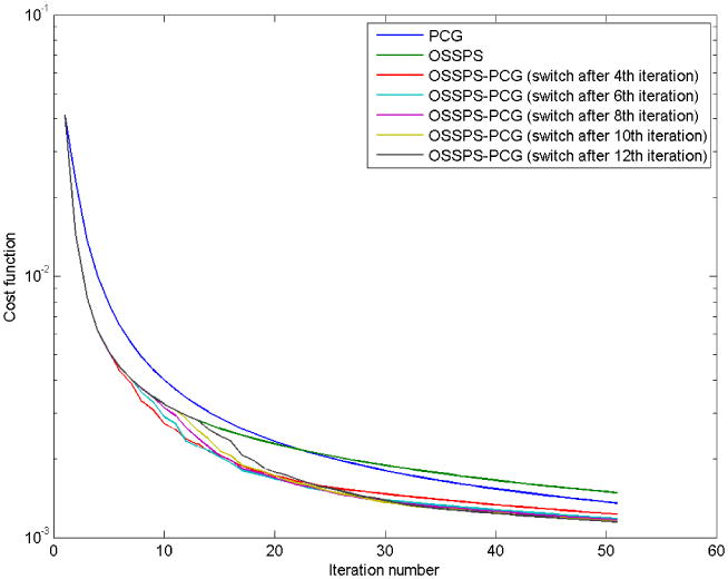
Comparison of convergence curves of PCG, OSSPS, and OSSPS-PCG with the transition fromOSSPS to PCG occurring after iteration numbers 4, 6, 8, 10, and 12. These curves were obtained for the L¹-TV penalty and for a random initialization. For OSSPS, one complete cycle through all the subsets is considered one iteration.

3. Results

We tested the joint L¹ and TV regularization approach and compared it with the L¹, TV, and L² penalties using simulated and experimental data. In this section, we describe the experimental setup, present some simulations based on a setup similar to the experimental setup, evaluate the different penalties on the basis of some performance metrics, and, finally, present reconstruction results for experimental data.

3.1. Experimental setup

We acquired data using a mouse-shaped phantom. The experimental and computational steps leading up to the inverse problem are described below:

3.1.1. Phantom description

The mouse-shaped phantom (shown in figure 2(a)) was made using a mold created from a euthanized mouse. The phantom material consisted of 1% Intralipid, 2% agar, and 20 μM hemoglobin (Li et al. 2009). Two transparent capillary tubes, each 20 mm long, 1 mm in diameter, and filled with 1 μM DiD solution (D307, Invitrogen Corporation, excitation peak 648 nm, emission peak 669 nm, http://products.invitrogen.com/ivgn/product/D307), were embedded inside the mouse-shaped phantom. The embedded line sources are visible in the CT image, shown in figure 2(b).

Figure 2.

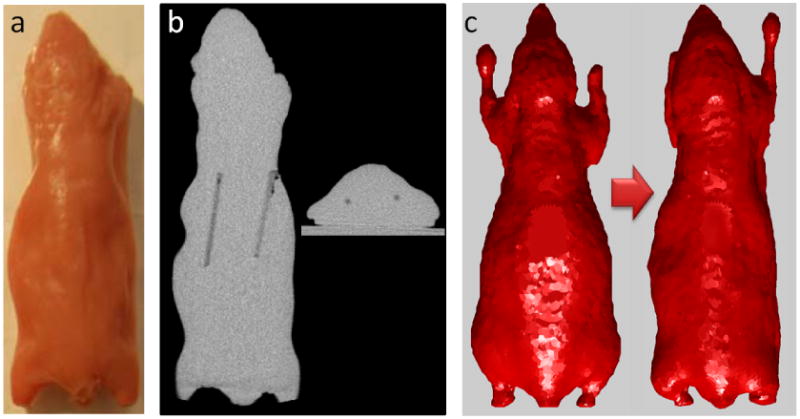
Mouse-shaped phantom. (a) Full-light photograph. (b) A coronal and a transverse section from the CT image showing the two tubes filled with fluorescent DiD dye. (c) Original and warped Digimouse surfaces.

3.1.2. Data acquisition

Surface fluorescence data was collected using an FMT imaging setup equipped with an EMCCDcamera for image acquisition and a conical mirror for full surface viewing (Li et al. 2009) shown in figure 3(a). The excitation source was a 650 nm laser beam focused to spots of ∼1 mm diameter on the surface of the phantom. A pair of motorized mirrors was used to direct the beam to 54 different locations scattered nonuniformly over the surface of the phantom (as shown in figure 3). Fluorescence data was collected at an emission wavelength of 720 nm. MicroCT scans of the phantom were obtained on an Inveon MM system (Siemens Preclinical Solutions). 180 angular projections were acquired over 360° with an X-ray tube voltage of 80 kVp and current of 0.3 mA. Images were reconstructed using the filtered backprojection algorithm with a voxel size of 0.097732 mm.

Figure 3.

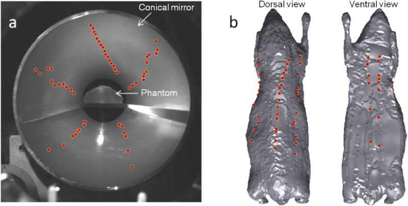
(a) Full-light EMCCD camera image showing the mouse phantom seated on a stage with its full surface visible in the conical mirror. The dots represent the 54 illumination locations as seen in the image space. (b) Dorsal and ventral views of the tessellated mouse phantom showing the illumination points mapped to the object space.

3.1.3. Data preprocessing

The mapping of the fluorescence data from the CCD camera images to the phantom surface requires a digital volumetric representation of the phantom. We used the Digimouse atlas (http://neuroimage.usc.edu/Digimouse.html) (Dogdas et al. 2007, Stout et al. 2002), a labeled atlas, based on co-registered CT and cryosection images of a 28 g normal male nude mouse. We first extracted the surface geometry of the phantom from its CT image. We then used the DigiWarp technique (Joshi et al. 2009, Joshi et al. 2010) to warp the Digimouse atlas to fit the extracted phantom surface. The original and warped Digimouse surfaces are shown in figure 2(c). The fluorescence data was then mapped to the warped atlas surface using a calibrated mapping technique developed for the conical mirror based imaging system (Dutta 2011).

3.1.4. Forward model generation

The warped Digimouse atlas, with 306,771 tetrahedrons and 58,244 tessellation nodes, was used to solve the forward problem. We first used the finite element method to compute theexcitation and emission forward model matrices, A^ex ∈ ^n_s×n_d and A^em ∈^n_d×n_s, for n_d = 6,762 surface detector nodes and n_s = 11, 036 volumetric grid points and for excitation and emission wavelengths of 650 nm and 720 nm respectively. The volumetric grid points with a uniform spacing of 1 mm represent the source spacefor reconstruction. Next, A^ex was used to compute the excitation fields, ${\mathit{\text{D}}}_{\mathit{\text{k}}}^{\mathit{\text{ex}}}$, k being the pattern index, for all the 54 patterns. Owing to the large size of the forward model matrix, A, as revealed by (29), it is important to avoid its direct computation. Instead, we use its building blocks – A^em and the ${\mathit{\text{D}}}_{\mathit{\text{k}}}^{\mathit{\text{ex}}}$ matrices – to efficiently compute forward- and backprojections given by:

$$\mathit{\text{Ax}}=\left[\begin{array}{c}{\mathit{\text{A}}}^{\mathit{\text{em}}}\left({\mathit{\text{d}}}_1^{\mathit{\text{ex}}}\circ \mathit{\text{x}}\right)\\ {\mathit{\text{A}}}^{\mathit{\text{em}}}\left({\mathit{\text{d}}}_2^{\mathit{\text{ex}}}\circ \mathit{\text{x}}\right)\\ ⋮\\ {\mathit{\text{A}}}^{\mathit{\text{em}}}\left({\mathit{\text{d}}}_p^{\mathit{\text{ex}}}\circ \mathit{\text{x}}\right)\end{array}\right]$$ (33)

$${\mathit{\text{A}}}^{\prime }\mathit{\text{y}}=\sum _k{\mathit{\text{d}}}_k^{\mathit{\text{ex}}}\circ \left({\left({\mathit{\text{A}}}^{\mathit{\text{em}}}\right)}^{\prime }{\mathit{\text{y}}}_k\right),$$ (34)

where x ∈ ^n_s and y ∈ ^n_dp are arbitrary vectors, ${\mathit{\text{d}}}_{\mathit{\text{k}}}^{\mathit{\text{ex}}}$ is a vector containing the diagonal terms of ${\mathit{\text{D}}}_{\mathit{\text{k}}}^{\mathit{\text{ex}}}$, and y_k is the kth block of y such that $\mathit{\text{y}}=[{y^{\prime }}_1{{\mathit{\text{y}}}^{\prime }}_2\dots {{\mathit{\text{y}}}^{\prime }}_p]\prime$.

3.2. Simulation results

We simulated two fluorescent line sources inside the warped Digimouse atlas. The excitation and emission wavelengths were assumed to be 650 nm and 720 nm respectively – the same used in the experiment. The same 54 illumination locations from the experiment were used for excitation. White Gaussian noise with an SNR of 5 was added to the fluorescence data to make the simulations realistic. Coronal sections of the warped mouse atlas indicating the positions of the two simulated line sources are shown in figure 4(a). With joint L¹ and TV penalties, there are two regularization parameters to be selected. These parameters were empirically determined by sweeping them over a range of values. The result of this study is presented in figure 5, where a coronal slice from the reconstructed image is shown for different combinations of values for these two parameters. We use values of 10⁻⁵, 5 × 10⁻⁵, and 2.5 × 10⁻⁴ for λ_L1 and 4 × 10⁻⁷, 2 × 10⁻⁶, and 10⁻⁵ for λ_TV. This figure clearly indicates the increasing sparsifying and smoothing effects as we increase the weights on the L¹ and TV penalties respectively. Based on this study, we pick intermediate values of 5 × 10⁻⁵ for λ_L1 and 2 × 10⁻⁶ for λ_TV. Figures 4(b), (c), (d), and (e) show full slice-by-slice reconstruction results for L², L¹, TV, and joint L¹-TV penalties respectively for indicated regularization parameters.

Figure 4.

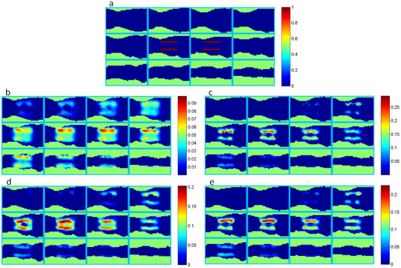
Simulated mouse phantom: coronal sections of the mouse phantom showing (a) the two simulated line sources and the reconstruction result for (b) the L² penalty with a regularization parameter of 10⁻³, (c) the L¹ penalty with a regularization parameter of 5×10⁻⁵, (d) the TV penalty with a regularization parameter of 2×10⁻⁶, and (e) both L¹ and TV penalties with regularization parameters of 5 × 10⁻⁵ and 2 × 10⁻⁶ respectively. The slices are ordered from bottom to top starting top left inthe image and ending bottom right.

Figure 5.

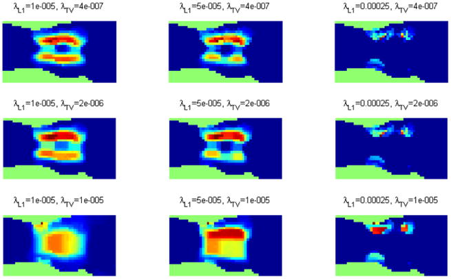
Reconstructed source distribution for different combinations of the L¹ and TV regularization parameters shown for a central coronal section from the phantom. These images demonstrate the sparsifying and smoothing effects of the L¹ and TV terms respectively.

We used 6 noisy realizations of the described simulation setup to compute a set of metrics for evaluating the different regularization schemes. The fluorescence data was corrupted using Gaussian noise with an SNR of 1. The regularization parameters used are λ_L2 = 10⁻³, λ_L1 = 5 × 10⁻⁵, and λ_TV = 2 × 10⁻⁶ (same as in figure 4). The computed metrics include the mean squared error (MSE), the mean and standard deviation of the signal over the region of interest (ROI), the mean and standard deviation of the background signal, and, finally, the signal-to-background ratio (SBR), defined as the ratio of the ROI mean to the background mean. The ROI is defined as the region consisting of voxels with a signal level of 1, corresponding to the two line sources in figure 4(a). The remaining voxels with zero signal comprise the background. These performance metrics for the different penalties are shown in figure 6. The joint L¹-TV penalty was observed to yield the lowest MSE value. The L¹, TV, and the joint L¹-TV schemes led to stronger mean signal levels over the ROI than the L². The L¹ and the joint L¹-TV approaches generated the least mean background signal level, while the joint L¹-TV approach yielded a lower background standard deviation than the L¹ and TV penalties individually. Lastly, the joint L¹-TV scheme offered an SBR in between those for the L¹ and TV penalties individually, while all of these three schemes had an SBR significantly better than that for the L² penalty.

Figure 6.

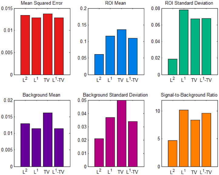
Performance metrics for comparison of the L², L¹, TV, and joint L¹ and TV penalty functions.

3.3. Experimental results

We reconstructed the experimental data acquired using the setup described in section 3.1 using the L², L¹, TV, and joint L¹-TV penalties. The results are shown in figures 7(a), (b), (c), and (d) respectively for indicated regularization parameters. The result obtained using the joint L¹-TV regularization scheme is overlaid against the CT image and displayed in figure 8. The two images were registered and displayed using the AMIDE tool for viewing and analyzing medical imaging data (Loening and Gambhir 2003). We observe a reasonable degree of overlap between the reconstructed FMT image and the ground truth revealed by the CT image.

Figure 7.

Experimental mouse phantom: coronal sections of the mouse phantom showing the reconstruction of two embedded line sources using (a) the L² penalty with a regularization parameter of 10⁻⁴, (b) the L¹ penalty with a regularization parameter of 20, (c) the TV penalty with a regularization parameter of 0.5, and (d) both L¹ and TV penalties with regularization parameters of 10 and 1 respectively.

Figure 8.

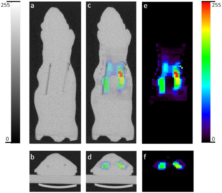
(a) Coronal and (b) transverse sections of the CT image of the mouse-shaped phantom showing the two embedded fluorescent line sources. (c) Coronal and (d) transverse overlay of CT and FMT images. (e) Coronal and (f) transverse sections of the FMT image showing thetwo fluorescent line sources reconstructed using both L¹ and TV penalties with regularization parameters of 10 and 1 respectively.

The performance metrics used to evaluate the simulation results utilize quantitative knowledge of the ground truth as well as multiple noise realizations. While the CT image contains information about the location of the capillary tubes, it does not provide the true intensities of the targets. We, therefore, are unable to directly apply the same set of performance metrics to the experimental study. Instead, we resort to the Dice similarity coefficient (Dice 1945), a spatial similarity index, for quantitative evaluation of the experimental results. The CT image was first blurred using a Gaussian kernel with full width at half maximum of 4 mm to make the resolutions of the two modalities comparable. Intensity based segmentation was then performed on the blurred CT image as well as the reconstructed FMT images. A numeric label i ∈ {1, 2, 3} was assigned to each image voxel, i = 1 representing target 1 (the line source to the right in figure 8), i = 2 representing target 2 (the line source to the left in figure 8), and i = 3 representing the background. The Dice similarity coefficient, d, was then computed as:

$$d=\frac{2\left|I_{\mathit{\text{CT}}}^i\cap I_{\mathit{\text{FMT}}}^i\right|}{\left|I_{\mathit{\text{CT}}}^i\right|+\left|I_{\mathit{\text{FMT}}}^i\right|},$$ (35)

where $I_{\mathit{\text{CT}}}^i$ and $I_{\mathit{\text{FMT}}}^i$ represent the sets of voxel indices that carry label i in the CT and FMT images respectively and the notation |.| represents the cardinality of a set. The value of d ranges from 0, indicating no spatial overlap between the two sets, to 1, indicating complete overlap. The results, shown in figure 9, indicate that the L² and the joint L¹-TV penalties perform consistently well for all three segments while the relative performance of the individual L¹ and TV penalties varies.

Figure 9.

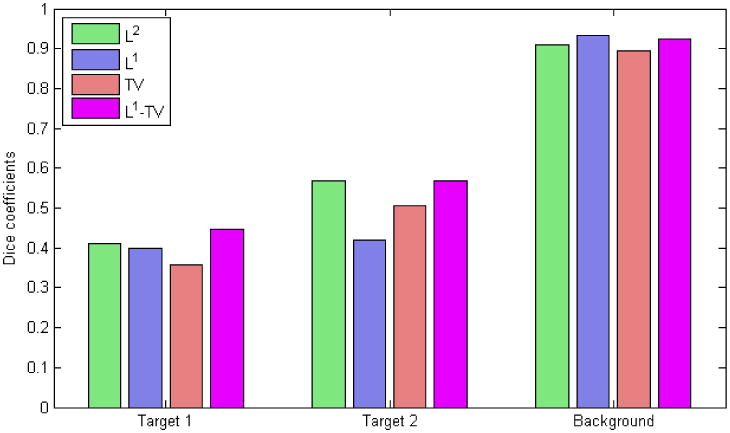
Dice coefficients representing the similarity between the CT image and the reconstructed FMT images for different penalties. Target 1 represents the line source to the right in all the subimages in figure 8 while target 2 represents the line source to the left.

4. Summary and Discussion

We have applied a combination of L¹ and TV penalties to the FMT inverse problem to simultaneously encourage properties of sparsity and smoothness in our reconstructed images. We derived inspiration from the fact that very often fluorescent probes and contrast agents are concentrated within specific areas of interest (e.g., inside localized tumors and excretory organs). We have presented a compound method that uses a combination of OSSPS and PCG algorithms to generate a convergent solution.

Exploiting the non-negativity constraint, we substituted the L¹ norm penalty with a linear term. SPS functions were derived for the data-fitting term and the TV penalty. While the MM algorithm guarantees monotonicity, the OS approach that was incorporated to increase convergence speed does not guarantee convergence. Typically this is handled by using a diminishing step size. But our compound approach, where the final solution is obtained using PCG, guarantees convergence. This approach was inspired by the observation that, far away from the solution, the SPS-OS method has a faster rate of convergence, while PCG is faster in the vicinity of the solution. The advantage of the OSSPS approach over PCG is that it eliminates the need for an expensive line search and requires fewer numbers of flops per iteration. On a 2.93 GHz Intel^® Core i7 CPU, it took about 40 s to complete one iteration of PCG while it took about 20 s to cycle through all 5 subsets and complete one iteration of OSSPS. 5 data blocks were used for the OS implementation, and the order of the blocks was chosen randomly at the start of the optimization procedure.

We validated the derived procedure using simulated and experimental data based on a mouse-shaped phantom with two embedded line sources. The simulation results showed that the L¹, TV, and joint L¹-TV penalties generated lower MSE values, stronger ROI mean signal levels, and higher SBR values than the L² regularizer. The joint L¹-TV approach generated a smooth solution with a sparse background. The joint L¹-TV result had the least mean background signal level and a lower background standard deviation than the L¹ and TV penalties individually. The L¹-TV reconstructed image obtained from experimental data was qualitatively validated by overlaying it against a CT image of the phantom. Quantitative evaluation of the experimental results was performed by computing Dice similarity coefficients between the FMT images and the CT image blurred to a similar resolution.

While the simulation and experimental setups appear similar, they are not identical. The only sources of inaccuracy in simulation are noise and numerical errors due to the ill-conditioning of the system matrix. In comparison, the experimental results are susceptible to a number of nonidealities arising from imperfect modeling and registration. These include incorrect estimates of optical properties, inaccuracies in the noise model, geometric and radiometric calibration errors associated with the imaging system, and imperfect alignment of the CT-derived surface in the FMT object space – amongst other factors. Unlike the experimental procedure which is subject to such uncertainties, the simulation setup allows us to focus exclusively on the relative merits of the reconstruction schemes.

Additionally, the illumination setup used consisted of a group of point excitation locations nonuniformly scattered over the surface. The suboptimality of this configuration leads to significant variations in sensitivity over different volumetric locations. A manifestation of this can be found in the marked difference between the reconstruction quality of the two fluorescence targets – in both simulation and experimental results. We may treat the squared L² norm of a column of the system matrix corresponding to particular voxel as a measure of the relative sensitivity of that voxel. The overall sensitivity (averaged over constituent voxels) is 3.9957 × 10⁻⁵ for target 1 (which appears brighter in the reconstructed images) and 1.1718 × 10⁻⁵ for target 2 (which appears fainter). Of the different penalties, the difference in the reconstruction quality between the two targets is perhaps least pronounced in the TV case. This is due to the inherent tendency of the TV penalty to promote piecewise constancy.

Using L¹ or TV regularization, in combination or separately, clearly leads to improvements in localizing fluorescent sources in FMT in cases where the true distribution is consistent with the assumptions implicit in using these regularizers. There is less difference between the L¹, TV and, joint L¹-TV schemes than between any of these and L². Qualitatively, the joint L¹-TV images had the most natural appearance in the simulation and phantom studies we performed, but the quantitative studies reported in figure 6 do not identify a clear winner. As a final note, we observe that even with the use of these regularizers, FMT struggles to produce 3D images with resolutions that are routine in small animal PET and SPECT studies. This is because the FMT inverse problem is inherently more ill-posed, a situation which is exacerbated by uncertainties in the forward model. While the radiative transfer equation (Klose et al. 2005) models photon propagation more accurately than the diffusion equation (used in this work), it adds to the uncertainty by assuming prior knowledge of tissue anisotropies and also poses a significant computational challenge. The use of a larger number of illumination/detection wavelengths or a more optimal set of spatial patterns for illumination may lead to further improvements provided they improve the conditioning of the forward model.

References

- Ahn S, Fessler J. Globally convergent image reconstruction for emission tomography using relaxed ordered subsets algorithms. Medical Imaging, IEEE Transactions. 2003;22(5):613–626. doi: 10.1109/TMI.2003.812251. [DOI] [PubMed] [Google Scholar]
- Axelsson J, Svensson J, Andersson-Engels S. Spatially varying regularization based on spectrally resolved fluorescence emission in fluorescence molecular tomography. Optics Express. 2007;15(21):13574–13584. doi: 10.1364/oe.15.013574. [DOI] [PubMed] [Google Scholar]
- Beck A, Teboulle M. A fast iterative shrinkage-thresholding algorithm for linear inverse problems. SIAM Journal on Imaging Sciences. 2009;2(1):183–202. [Google Scholar]
- Bélanger S, Abran M, Intes X, Casanova C, Lesage F. Real-time diffuse optical tomography based on structured illumination. Journal of Biomedical Optics. 2010;15:016006. doi: 10.1117/1.3290818. [DOI] [PubMed] [Google Scholar]
- Bertsekas DP. Nonlinear Programming. Athena Scientific; 1999. [Google Scholar]
- Bloch S, Lesage F, McIntosh L, Gandjbakhche A, Liang K, Achilefu S. Whole-body fluorescence lifetime imaging of a tumor-targeted near-infrared molecular probe in mice. Journal of Biomedical Optics. 2005;10(5):054003. doi: 10.1117/1.2070148. [DOI] [PubMed] [Google Scholar]
- Candes EJ, Wakin MB. An introduction to compressive sampling. Signal Processing Magazine, IEEE. 2008;25(2):21–30. [Google Scholar]
- Cao N, Nehorai A, Jacobs M. Image reconstruction for diffuse optical tomography using sparsity regularization and expectation-maximization algorithm. Optics Express. 2007;15(21):13695–13708. doi: 10.1364/oe.15.013695. [DOI] [PubMed] [Google Scholar]
- Chambolle A. An algorithm for total variation minimization and applications. Journal of Mathematical Imaging and Vision. 2004;20:89–97. [Google Scholar]
- Chan T, Golub G, Mulet P. A nonlinear primal-dual method for total variation-based image restoration. ICAOS'96. 1996:241–252. [Google Scholar]
- Chaudhari AJ, Ahn S, Levenson R, Badawi RD, Cherry SR, Leahy RM. Excitation spectroscopy in multispectral optical fluorescence tomography: methodology, feasibility and computer simulation studies. Physics in Medicine and Biology. 2009;54(15):4687–4704. doi: 10.1088/0031-9155/54/15/004. [DOI] [PMC free article] [PubMed] [Google Scholar]
- Chen SS, Donoho DL, Saunders MA. Atomic decomposition by basis pursuit. SIAM Journal on Scientific Computing. 1998;20(1):33–61. [Google Scholar]
- Daubechies I, Friese MD, Mol CD. Communications in Pure and Applied Mathematics. 2004. An iterative thresholding algorithm for linear inverse problems with a sparsity constraint; p. 14131457. [Google Scholar]
- Dice L. Measures of the amount of ecologic association between species. Ecology. 1945;26(3):297–302. [Google Scholar]
- Dogdas B, Stout D, Chatziioannou A, Leahy RM. Digimouse: A 3D whole body mouse atlas from CT and cryosection data. Physics in Medicine and Biology. 2007;52:577–587. doi: 10.1088/0031-9155/52/3/003. [DOI] [PMC free article] [PubMed] [Google Scholar]
- Donoho DL. Compressed sensing. Information Theory, IEEE Transactions. 2006;52(4) [Google Scholar]
- Dutta J. PhD thesis. University of Southern California; Los Angeles, California: 2011. Computational methods for fluorescence molecular tomography. [Google Scholar]
- Dutta J, Ahn S, Joshi AA, Leahy RM. ‘Biomedical Imaging: From Nano to Macro ISBI ’ 09 IEEE International Symposium on'. 2009. Optimal illumination patterns for fluorescence tomography; pp. 1275–1278. [DOI] [PMC free article] [PubMed] [Google Scholar]
- Dutta J, Ahn S, Joshi AA, Leahy RM. Illumination pattern optimization for fluorescence tomography: theory and simulation studies. Physics in Medicine and Biology. 2010;55(10):2961. doi: 10.1088/0031-9155/55/10/011. [DOI] [PMC free article] [PubMed] [Google Scholar]
- Dutta J, Ahn S, Li C, Chaudhari AJ, Cherry SR, Leahy RM. Medical Imaging 2008: Physics of Medical Imaging. Vol. 6913. SPIE; 2008. Computationally efficient perturbative forward modeling for 3D multispectral bioluminescence and fluorescence tomography; p. 69130C. [Google Scholar]
- Efron B, Hastie T, Johnstone I, Tibshirani R. Least angle regression. The Annals of Statistics. 2004;32(2):407–499. [Google Scholar]
- Eppstein MJ, Hawrysz DJ, Godavarty A, Sevick-Muraca EM. Three-dimensional, Bayesian image reconstruction from sparse and noisy data sets: Near-infrared fluorescence tomography. Proceedings of the National Academy of Sciences. 2002;99(15):9619–9624. doi: 10.1073/pnas.112217899. [DOI] [PMC free article] [PubMed] [Google Scholar]
- Erdogan H, Fessler JA. Ordered subsets algorithms for transmission tomography. Physics in Medicine and Biology. 1999;44(11):2835–2851. doi: 10.1088/0031-9155/44/11/311. [DOI] [PubMed] [Google Scholar]
- Fessler JA, Clinthorne NH, Rogers WL. Regularized emission image reconstruction using imperfect side information. Nuclear Science, IEEE Transactions. 1992;39(5):1464–1471. [Google Scholar]
- Fessler JA, Hero AOI. Penalized maximum-likelihood image reconstruction using space-alternating generalized EM algorithms. Image Processing, IEEE Transactions. 1995;4(10):1417–1429. doi: 10.1109/83.465106. [DOI] [PubMed] [Google Scholar]
- Figueiredo MAT, Nowak RD, Wright SJ. Gradient projection for sparse reconstruction: Application to compressed sensing and other inverse problems. Selected Topics in Signal Processing, IEEE Journal. 2007;1(4):586–597. [Google Scholar]
- Gao H, Zhao H. Multilevel bioluminescence tomography based on radiative transfer equation part 1: L1 regularization. Optics Express. 2010a;18(3):1854–1871. doi: 10.1364/OE.18.001854. [DOI] [PubMed] [Google Scholar]
- Gao H, Zhao H. Multilevel bioluminescence tomography based on radiative transfer equation part 2: total variation and L1 data fidelity. Optics Express. 2010b;18(3):2894–2912. doi: 10.1364/OE.18.002894. [DOI] [PubMed] [Google Scholar]
- Gardner C, Dutta J, Mitchell GS, Ahn S, Li C, Harvey P, Gershman R, Sheedy S, Mansfield J, Cherry SR, Leahy RM, Levenson R. Biomedical Optics, OSA Technical Digest (CD) (Optical Society of America, 2010) OSA: Paper BTuF1; 2010. Improved in vivo fluorescence tomography and quantitation in small animals using a novel multiview, multispectral imaging system. [Google Scholar]
- Green PJ. Bayesian reconstructions from emission tomography data using a modified EM algorithm. Medical Imaging, IEEE Transactions. 1990;9(1):84–93. doi: 10.1109/42.52985. [DOI] [PubMed] [Google Scholar]
- Guven M, Yazici B, Intes X, Chance B. Diffuse optical tomography with a priori anatomical information. Physics in Medicine and Biology. 2005;50(12):2837. doi: 10.1088/0031-9155/50/12/008. [DOI] [PubMed] [Google Scholar]
- Hebert T, Leahy RM. A generalized EM algorithm for 3-D Bayesian reconstruction from Poisson data using Gibbs priors. Medical Imaging, IEEE Transactions. 1989;8(2):194–202. doi: 10.1109/42.24868. [DOI] [PubMed] [Google Scholar]
- Huang Y, Ng MK, Wen YW. A fast total variation minimization method for image restoration. Multiscale Modeling & Simulation. 2008;7(2):774–795. [Google Scholar]
- Hyde D, Miller EL, Brooks DH, Ntziachristos V. Data specific spatially varying regularization for multimodal fluorescence molecular tomography. Medical Imaging, IEEE Transactions. 2010;29(2):365–374. doi: 10.1109/TMI.2009.2031112. [DOI] [PubMed] [Google Scholar]
- Joshi AA, Chaudhari AJ, Li C, Dutta J, Cherry SR, Shattuck DW, Toga AW, Leahy RM. DigiWarp: a method for deformable mouse atlas warping to surface topographic data. Physics in Medicine and Biology. 2010;55(20):6197. doi: 10.1088/0031-9155/55/20/011. [DOI] [PMC free article] [PubMed] [Google Scholar]
- Joshi AA, Chaudhari AJ, Li C, Shattuck D, Dutta J, Leahy RM, Toga AW. Biomedical Imaging: From Nano to Macro, 2009 ISBI '09 IEEE International Symposium on. 2009. Posture matching and elastic registration of a mouse atlas to surface topography range data; pp. 366–369. [DOI] [PMC free article] [PubMed] [Google Scholar]
- Joshi A, Bangerth W, Sevick-Muraca EM. Non-contact fluorescence optical tomography with scanning patterned illumination. Optics Express. 2006;14(14):6516–6534. doi: 10.1364/oe.14.006516. [DOI] [PubMed] [Google Scholar]
- Kim SJ, Koh K, Lustig M, Boyd S, Gorinevsky D. An interior-point method for large-scale l1-regularized least squares. Selected Topics in Signal Processing, IEEE Journal. 2007;1(4):606–617. [Google Scholar]
- Klose A, Ntziachristos V, Hielscher A. The inverse source problem based on the radiative transfer equation in optical molecular imaging. Journal of Computational Physics. 2005;202(1):323–345. [Google Scholar]
- Lange K. Convergence of em image reconstruction algorithms with Gibbs smoothing. Medical Imaging, IEEE Transactions. 1990;9(4):439–446. doi: 10.1109/42.61759. [DOI] [PubMed] [Google Scholar]
- Lange K, Fessler JA. Globally convergent algorithms for maximum a posteriori transmission tomography. Image Processing, IEEE Transactions. 1995;4(10):1430–1438. doi: 10.1109/83.465107. [DOI] [PubMed] [Google Scholar]
- Lange K, Hunter DR, Yang I. Optimization transfer using surrogate objective functions. Journal of Computational and Graphical Statistics. 2000;9(1):1–20. [Google Scholar]
- Leahy RM, Yan X. Information Processing in Medical Imaging. In: Colchester A, Hawkes D, editors. Lecture Notes in Computer Science. Vol. 511. Springer Berlin; Heidelberg: 1991. pp. 105–120. [Google Scholar]
- Li A, Boverman G, Zhang Y, Brooks D, Miller EL, Kilmer ME, Zhang Q, Hillman EMC, Boas DA. Optimal linear inverse solution with multiple priors in diffuse optical tomography. Applied Optics. 2005;44(10):1948–1956. doi: 10.1364/ao.44.001948. [DOI] [PubMed] [Google Scholar]
- Li C, Mitchell GS, Dutta J, Ahn S, Leahy RM, Cherry SR. A three-dimensional multispectral fluorescence optical tomography imaging system for small animals based on a conical mirror design. Optics Express. 2009;17(9):7571–7585. doi: 10.1364/oe.17.007571. [DOI] [PMC free article] [PubMed] [Google Scholar]
- Li Q, Ahn S, Leahy RM. Fast hybrid algorithms for PET image reconstruction. Nuclear Science Symposium Conference Record, 2005 IEEE. 2005;4:390–393. [Google Scholar]
- Loening A, Gambhir S. AMIDE: a free software tool for multimodality medical image analysis. Molecular Imaging. 2003;2(3):131–137. doi: 10.1162/15353500200303133. [DOI] [PubMed] [Google Scholar]
- Massoud TF, Gambhir SS. Molecular imaging in living subjects: seeing fundamental biological processes in a new light. Genes & Development. 2003;17(5):545–580. doi: 10.1101/gad.1047403. [DOI] [PubMed] [Google Scholar]
- Mohajerani P, Eftekhar AA, Huang J, Adibi A. Optimal sparse solution for fluorescent diffuse optical tomography: theory and phantom experimental results. Applied Optics. 2007;46(10):1679–1685. doi: 10.1364/ao.46.001679. [DOI] [PubMed] [Google Scholar]
- Natarajan BK. Sparse approximate solutions to linear systems. SIAM Journal on Computing. 1995;24(2):227–234. [Google Scholar]
- Pogue BW, McBride TO, Prewitt J, Österberg UL, Paulsen KD. Spatially variant regularization improves diffuse optical tomography. Applied Optics. 1999;38(13):2950–2961. doi: 10.1364/ao.38.002950. [DOI] [PubMed] [Google Scholar]
- Rudin LI, Osher S, Fatemi E. Nonlinear total variation based noise removal algorithms. Physica D: Nonlinear Phenomena. 1992;60(1–4):259–268. [Google Scholar]
- Shu X, Royant A, Lin MZ, Aguilera TA, Lev-Ram V, Steinbach PA, Tsien RY. Mammalian Expression of Infrared Fluorescent Proteins Engineered from a Bacterial Phytochrome. Science. 2009;324(5928):804–807. doi: 10.1126/science.1168683. [DOI] [PMC free article] [PubMed] [Google Scholar]
- Stout D, Chow P, Silverman R, Leahy RM, Lewis X, Gambhir S, Chatziioannou A. Creating a whole body digital mouse atlas with PET, CT and cryosection images. Molecular Imaging and Biology. 2002;4(4):S27. [Google Scholar]
- Strong D, Chan T. Edge-preserving and scale-dependent properties of total variation regularization. Inverse Problems. 2003;19(6):S165. [Google Scholar]
- Tibshirani R. Regression shrinkage and selection via the Lasso Journal of the Royal Statistical Society. Series B (Methodological) 1996;58(1):267–288. [Google Scholar]
- Tikhonov AN, Arsenin VY. Solutions of Ill-Posed Problems. John Wiley & Sons; Washington, D.C: 1977. [Google Scholar]
- Vogel C, Oman M. Iterative methods for total variation denoising. SIAM Journal on Scientific Computing. 1996;17(1):227–238. [Google Scholar]
- Vogel CR, Oman ME. Fast, robust total variation-based reconstruction of noisy, blurred images. Image Processing, IEEE Transactions. 1998;7(6):813–824. doi: 10.1109/83.679423. [DOI] [PubMed] [Google Scholar]
- Weissleder R, Ntziachristos V. Shedding light onto live molecular targets. Nature Medicine. 2003;9:123–128. doi: 10.1038/nm0103-123. [DOI] [PubMed] [Google Scholar]
- Weissleder R, Tung CH, Mahmood U, Bogdanov A. In vivo imaging of tumors with protease-activated near-infrared fluorescent probes. Nature Biotechnology. 1999;17(4):375–378. doi: 10.1038/7933. [DOI] [PubMed] [Google Scholar]
- Zacharakis G, Kambara H, Shih H, Ripoll J, Grimm J, Saeki Y, Weissleder R, Ntziachristos V. Volumetric tomography of fluorescent proteins through small animals in vivo. Proceedings of the National Academy of Sciences. 2005;102(51):1825218257. doi: 10.1073/pnas.0504628102. [DOI] [PMC free article] [PubMed] [Google Scholar]