Figure 4.

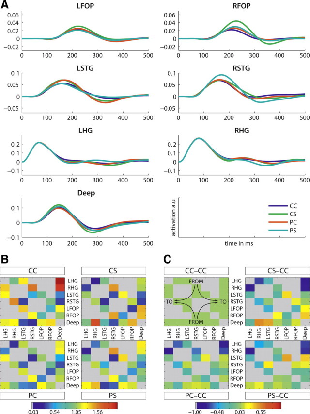
Time courses and connectivities of winning model families. A, Mean time courses of the winning families (all models that included a deep source). B, Bayesian model averages including models of the winning families (HG, STG, FOP): mean connectivity between all regions. Note the stronger connection (dark red) from the deep source to the cortical region (LHG)—right upper corner of the CC square. Blue means lowest connectivity. The redundant and nonexisting connections are displayed in gray. The panels display the values for the different conditions CC, CS, PC, and PS, respectively. Direction of connectivity is indicated in the CC-CC panel of part C: “from” is displayed at the top/bottom and “to” on the left/right. C, Bayesian model averages based on models of the winning families (HG, STG, FOP): difference in the mean connectivity between all regions to the condition CC. Note that green means difference equals zero. The redundant and nonexisting connections are displayed in gray. The upper left panel displays the values for condition CC-CC, the upper right panel—condition CS-CC, the lower left panel—condition PC-CC, and the lower right panel—condition PS-CC.