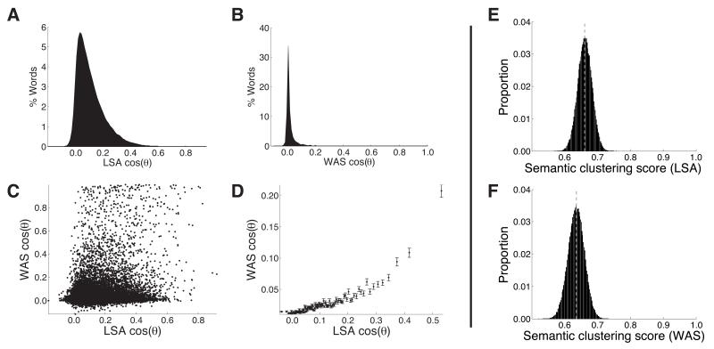
Figure 1. A. -D. Two measures of semantic similarity.
A. Distribution of the pairwise LSA-derived semantic similarity values for the words shown in Table 1. B. Distribution of the pairwise WAS-derived semantic similarity values for the same words. C. The panel shows a scatterplot comparing the LSA- and WAS-derived similarity values. Each dot corresponds to a single comparison between two words. Pearson’s correlation: r = 0.255, p < 10−3; Spearman’s correlation: ρ = 0.184, p < 10−3. D. This panel shows a binned variant of the scatterplot in panel C. We first divided the distributions of LSA-derived pairwise similarity values into 100 equally sized bins (the centers of the bins are plotted along the x-coordinate). The heights of each dot reflect the mean WAS-derived similarity values for the same pairs of words (error bars denote ± SEM). The binning reveals an approximately monotonic relation between the two similarity measures. Binned Pearson’s correlation: r = 0.875, p < 10−3; Spearman’s correlation: ρ = 0.954, p < 10−3. E., F. Semantic clustering simulations. E. We generated 5-item recall sequences that maximized the WAS-derived semantic clustering score for 100,000 simulated participants presented with 50 15-item lists each (see text for details). The panel shows the proportion of simulated participants that yielded the mean LSA-derived semantic clustering scores shown along the x-axis. F. This panel is identical to panel E, but here we generated recall sequences that maximized the LSA-derived semantic clustering scores, and plot the distribution of observed mean WAS-derived clustering scores. The same 5,000,000 randomly chosen 15-item lists were used in both panels. The dotted gray lines indicate the means of each distribution.

