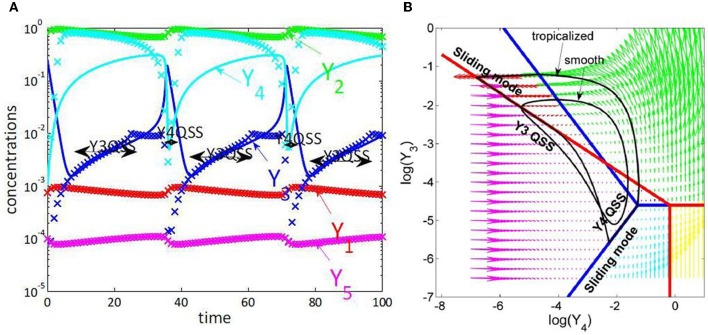
Figure 4.

Tropical geometry and cell cycle modeling. We considered the five variables cell cycle model defined by the differential equations y′₁ = k₉y₂ − k₈y₁ + k₆y₃, y′₂ = k₈y₁ − k₉y₂ − k₃y₂y₅, y′₃ = k′₄y₄ + k₄y₄y²₃/C² − k₆y₃, y′₄ = −k′₄y₄ − k₄y₄y²₃/C² + k₃y₂y₅, y′₅ = k₁ − k₃y₂y₅, proposed in Tyson (1991). (A) Comparison of trajectories and imposed trajectories show that variables y₁, y₂, y₅ are always slaved, meaning that the trajectories are close to the 2 dimensional hyperplane defined by the QE condition k₈y₁ = k₉y₂, the QSS condition k₁ = k₃y₂y₅ and the conservation law y₁ + y₂ + y₃ + y₄ = C. The variables y₃, y₄ are slaved and the corresponding species are quasi-stationary on intervals. This means that the dimensionality of the dynamics is further reduced to 1, on intervals. (B) Tropicalization on logarithmic paper, in the plane of the variables y₃, y₄. The tropical manifold consists of two tripods, represented in blue and red, which divide the logarithmic paper into six polygonal sectors. Monomial vector fields defining the tropicalized dynamics change from one polygonal domain to another. The tropicalized (approximated) and the smooth (not reduced) limit cycle dynamics stay within bounded distance one from another. This distance is relatively small on intervals where the variables y₃ or y₄ are quasi-stationary, which correspond to sliding modes of the tropicalization.