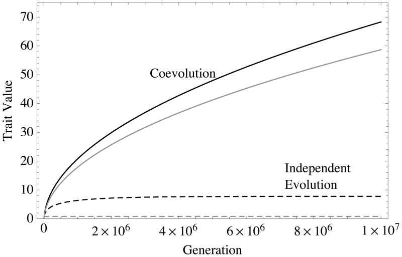
Figure 4. Evolutionary trajectories from numerical simulations.

Black curves denote phenotypic values of survival/fecundity helping, and gray curves denote resource-based helping. Dashed lines are trajectories for evolution of single-traits in the absence of the other trait (b_x = c_x = 0 for non-evolving trait x), while solid lines denote two-trait coevolutionary trajectories where both traits are allowed to coevolve in the same population. Single-trait evolution stalls at the ESS predicted by our analytical theory (see text and Fig. XX), while trait coevolution continues indefinitely. Simulation parameters are: F_ST = 0.5, ρ = 0.5, α = 0.1 (b_F = b_S = 0.1, c_F = c_S = 0.01 for coevolution), with initial conditions, S₀ = f₀ = 1, x_FS = 0.01, x_fs = 0.99, x_Fs = x_fS = 0 (see Appendix A for definitions). New beneficial mutations added when mutant allele frequency equals 0.99.