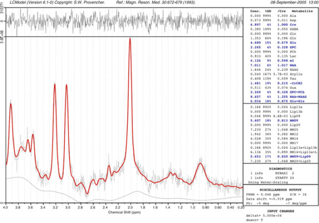
Fig. 9.11.

An example of the “LCModel” analysis method. The experimental data are fit as a linear combination of spectra of pure compounds recorded under the same experimental conditions as the in vivo spectrum. Automated baseline and phase correction is performed, and an estimate of metabolite concentrations provided relative to the brain water signal. In this example of a 2×2×2 cm PRESS spectrum recorded at 3.0 T from a normal control subject (TR/TE/number of averages = 2,000/35/128), the difference between the original data and the curve-fit (red) is shown in the top trace. Metabolite concentrations in blue correspond to those with an estimated uncertainty of less than 20%.