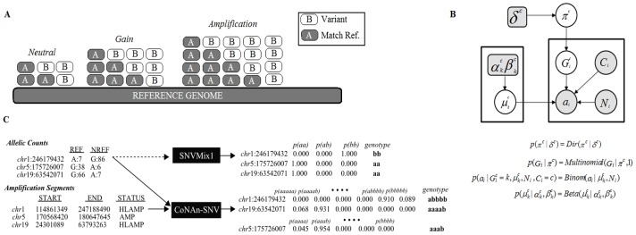
Figure 2. Overview of CoNAn-SNV model, inputs and outputs.

A) CoNAn-SNV genotype state-space expansion shown schematically. As higher levels of amplification are encountered, a larger genotype state-space is required to accommodate the different events that could arise due to amplifications (examples in Figure S1). B) CoNAn-SNV generative probabilistic graphical model. Circles represent random variables, and rounded squares represent fixed constants. Shaded nodes indicate observed data, such as allelic counts, while white nodes indicate quantities that are inferred during training though expectation maximisation. represents the CNA states of a segment (defined by the HMM describe in Shah et al. [6]) that spans position i; represents the genotype, which varies depending on CNA state; is the number of reads and is the number of reference reads; is prior existing over the genotypes and extends to accommodate CNA states; and is the genotype-specific Binomial parameter for genotype k in CNA state Ci. C) Example of CoNAn-SNV input and output. CoNAn-SNV takes allelic counts and as well is CNA segment data as input, while SNVMix requires only allelic counts. The same positions and counts are provided to both algorithms, with different results. In some cases CoNAn-SNV will call a variant with an aaaab or aaab genotype, which would otherwise be missed by SNVMix; also, however, CoNAn-SNV will also genotype a positions with abbbb rather than bb (as SNVMix [21] would), which allows for better interpretation of events.