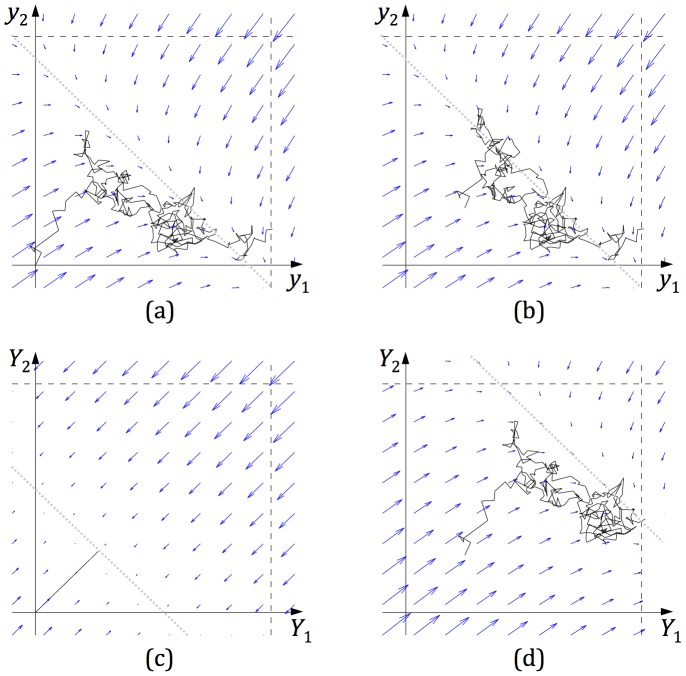
Figure 2. Dynamics of the mutual inhibition model ( equations A1 and A2 .
). In each panel the curve shows the evolution of the state of the model during a simulation, i.e. different points on the curve correspond to different time instances, and their co-ordinates correspond to levels of the activity of the accumulators at corresponding time. The simulations were performed using the Euler method with an integration constant of 0.001s. In all simulations k = w = 10, I 1 = 4,41, I 2 = 3, c = 0.33 (values of I 1, I 2, c were estimated from behaviour of a sample participant performing motion discrimination task as described in [13]) and the decision threshold was 0.4. The dashed lines indicate the positions in the state space in which one of the accumulators reaches a decision threshold. The arrows indicate the average direction in which the state moves from the point indicated by the arrow's tail, and its length corresponds to the speed of movement (i.e., rate of change) in the absence of noise. The dotted diagonal lines show the positions of the lines to which the state of the system is attracted. (a) Simulation of the model with y 1(0) = y 2(0) = 0. (b) Simulation of the model with y 1(0) = y 2(0) = 0.1. (c) Simulation of the model before stimulus onset (i.e. when I 1 = I 2 = c = 0). The simulation starts at Y 1(0) = Y 2(0) = 0, and the accumulators receive constant input I 0 = 2 for 1s. (d) Simulation of the model with Y 1(0) and Y 2(0) set to the last state in panel c, in which the accumulators receive additional constant input of I 0 = 2.

