Figure - PMC

Skip to main content

An official website of the United States government

Here's how you know

Here's how you know

Official websites use .gov
A .gov website belongs to an official government organization in the United States.

Secure .gov websites use HTTPS
A lock ( ) or https:// means you've safely connected to the .gov website. Share sensitive information only on official, secure websites.

View full-text article in PMC

. 2012 Aug 8;13:96. doi: 10.1186/1471-2202-13-96

Search in PMC
Search in PubMed
View in NLM Catalog
Add to search

Copyright ©2012 Oliynyk et al.; licensee BioMed Central Ltd.

This is an Open Access article distributed under the terms of the Creative Commons Attribution License ( http://creativecommons.org/licenses/by/2.0), which permits unrestricted use, distribution, and reproduction in any medium, provided the original work is properly cited.

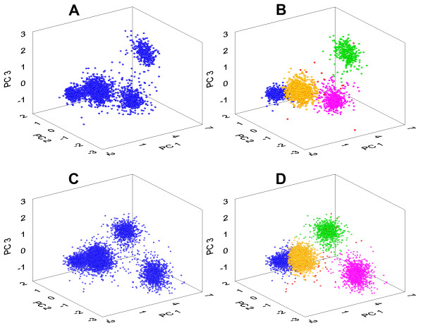
PMC Copyright notice

Rotable 3D scatter-plots of first three PC scores. The Figure shows an example automatic clustering of dataset A (fragments A and B are conditions before and after clustering analysis) and automatic classification of dataset B (fragments C and D are conditions before and after clustering). Each dot represents a spike situated in the 3D PC feature space. Four dense clusters are clearly visible and classified. Noise-near waveforms and their PCs located far away from cluster centres, as evaluated by Mahalanobis distance, are marked as red dots.