Fig. 6.

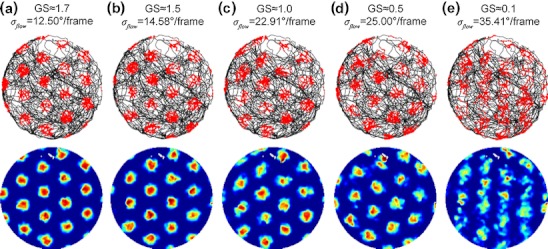
Examples for firing patterns of varying grid score (GS). The first row shows the different trajectories (black traces) with superimposed locations where a spike occurred (red dots). In the second row these spikes are registered in a 201 × 201 pixels image and are divided by the occupancy in these locations. Both registered spikes and occupancy are convolved with a squared Gaussian filter with nine pixels length and two pixels standard deviation. (a) A moderate amount of Gaussian flow noise (σ _flow = 12.5 °/frame) leads to a GS of 1.7. Increasing the amount of noise gives GS of 1.5 in (b), 1.0 in (c), 0.5 in (d), and 0.1 in (e). All values are for a reset interval of T _reset = 16.67 min and parameters of Gaussian flow noise σ _flow are given atop of each trajectory plot. The simulation uses the trajectory ‘Hafting_Fig2c_Trial1’ from Hafting et al. (2005). Note that the response patterns in the lower row are individually scaled to min (blue) and max (red) values of spikes per second. Regions plotted in white have never been visited, in this example the gap in direction “North”