Figure 6.

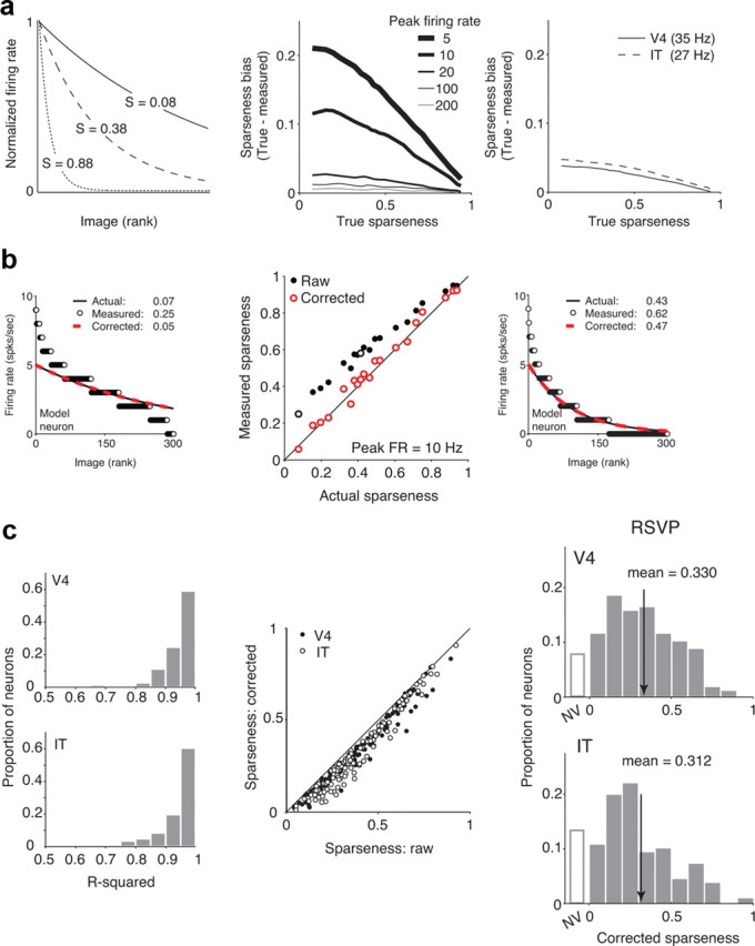
Sparseness biases arise from Poisson variability and can be corrected. a, Simulations illustrate that sparseness biases arise from Poisson variability. Left, Example exponential functions used to model neurons with the form R(x) = Ae^−αx, where A determines the peak firing rate, and α is inversely proportional to the steepness of response falloff. Sparseness values, calculated in the limit of infinite samples from these functions, are labeled. To simulate an experiment, 300 randomly selected points (hypothetical images) were sampled from an exponential with a fixed exponent (α) and peak rate (A), and five samples were randomly taken from a Poisson distribution centered at each mean to simulate five presentations of each image. Mean firing rates were calculated across the five trials, and sparseness is calculated as described previously (see Materials and Methods). Middle, Sparseness bias, calculated as the difference between the true sparseness and the sparseness measured in the simulated experiment, as a function of true sparseness. Sparseness is consistently overestimated, with the largest biases existing at low firing rates and low true sparseness. Right, Estimated sparseness biases at the mean firing rates recorded in the V4 and IT populations; although sparseness biases are expected to be large for neurons with low firing rates (middle), sparseness biases are expected to be small at the average firing rates observed across the population (bias < 0.05). To determine the degree to which these biases impact the results we report in Figure 3c, we developed a corrective procedure to estimate the true sparseness of each neuron (see Materials and Methods). b, Illustration of the bias correction procedure with model neurons. Left and right, Details of the bias correction for two example model neurons. Shown are the underlying exponential functions (black), the mean firing rate (FR) responses observed in a model experiment (white dots), and the recovered exponential after bias correction (red dashed line). Labeled are the actual, measured, and corrected sparseness values. Middle, Plot of measured versus actual sparseness based on raw data (black) and after the corrective procedure (red) for neurons with peak firing rates of 10 Hz. Open black circles indicate the two example model neurons shown. At all sparseness values, the correction improves the sparseness prediction. Thus, although this procedure is not guaranteed to perfectly recover the true sparseness of a neuron (e.g., noise in the original dataset cannot be removed), we found that this method was highly effective in estimating the true underlying exponential functions for model neurons. c, Corrective procedure applied to real data. Left, Histograms of the fraction of variance accounted for (r²) by the exponential model. Most cells were well described by an underlying exponential and Poisson variability (r² > 0.85: 95% of V4 and 87% of IT cells). Middle, Plot of corrected sparseness values as a function of raw (uncorrected values). Right, Histograms of corrected sparseness values for n = 142 V4 and n = 143 IT neurons. NV indicates neurons that did not respond significantly different than baseline to any of the 300 images (t test, p = 0.05). Means are indicated by arrows. V4 and IT distributions are shifted relative to their uncorrected values (compare with Fig. 3c) but remain statistically indistinguishable from one another (t test, p = 0.46; K–S test, p = 0.13).