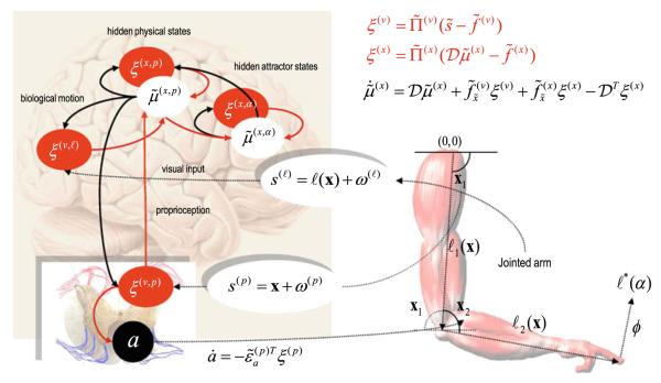
Fig. 1.

This schematic details the simulated mirror neuron system and the motor plant that it controls (left and right, respectively). The right panel depicts the functional architecture of the supposed neural circuits underlying active inference. The filled ellipses represent prediction error-units (neurons or populations), while the white ellipses denote state-units encoding conditional expectations about hidden states of the world. Here, they are divided into abstract attractor states (that supports stable heteroclinic orbits) and physical states of the arm (angular positions and velocities of the two joints). Filled arrows are forward connections conveying prediction errors and black arrows are backward connections mediating predictions. Motor commands are emitted by the black units in the ventral horn of the spinal cord. Note that these just receive prediction errors about proprioceptive states. These, in turn, are the difference between sensed proprioceptive input from the two joints and descending predictions from optimised representations in the motor cortex. The two jointed arm has a state space that is characterised by two angles, which control the position of the finger that will be used for writing in subsequent figures. The equations correspond to the expressions in the main text and represent a gradient decent on free-energy. They have been simplified here by omitting the hierarchical subscript and dynamics on hidden causes (which are not called on in this model)