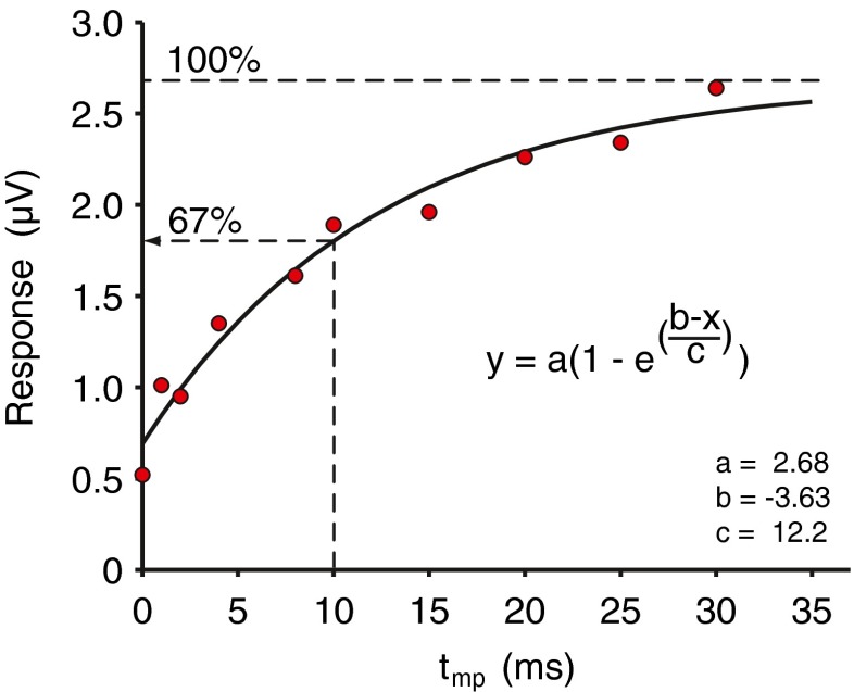
FIG. 6.

An example of a recovery curve derived with the NNFM paradigm. The amplitudes of the masked responses (red dots) are plotted as a function of ten different masker–probe intervals (t _mp) ranging from 0 to 30 ms. The conditions of the measurement were: nNW = 0, L _m = L _p = 40 dB SPL, f _p = 10 kHz. The solid curve is a fit through the data points using the formula in the figure with y the response and x the masker–probe interval. The parameters a, b, and c were determined using the Gauss–Newton method for nonlinear regression. The upper dashed line is the unmasked amplitude limit. The lower dashed line shows the fitted response value at t _mp = 10 ms, which is the value used in our standard paradigm.