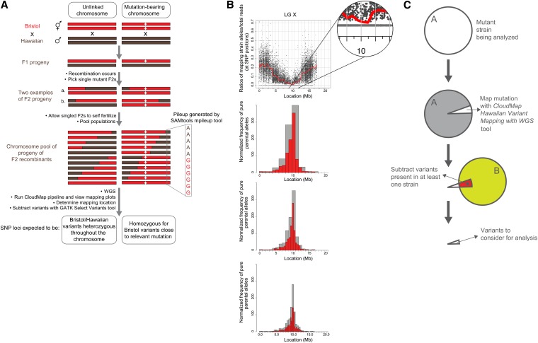
Figure 6 .

CloudMap Hawaiian Variant Mapping with WGS Data strategy. (A) Schematic presentation of a previously described one-step strategy for whole genome sequencing and mapping (Doitsidou et al. 2010) modeled on a similar strategy in plants (Schneeberger et al. 2009). (B) The CloudMap Hawaiian Variant Mapping With WGS tool plots the ratio of mapping strain alleles/total reads at each of the mapping strain SNP positions in the genome, as exemplified with the ot266 dataset. To better visualize trends in the scatter plots of the SNP ratios, we plot a LOESS regression line (red) through all the points on each chromosome. Each scatter plot also has a corresponding frequency plot that displays regions of linked chromosomes where pure parental allele SNP positions are concentrated. The same genomic region that shows linkage in the LOESS scatter plots also shows a matching peak in the frequency plots of pure parental alleles. These frequency plots are binned by default into 1-Mb (gray) and 0.5-Mb (red) bins although these bin sizes are adjustable. The figure also shows 2-Mb (gray) and 1-Mb (red) bin sizes (top frequency plot) and 0.5-Mb and 0.25-Mb bin sizes (bottom frequency plot). Data in these plots can also be normalized to improve the mapping signal (details in text, Figure 7, and Table S1). (C) CloudMap Hawaiian Variant Mapping with WGS Data variant subtraction. As described in the text and in Figure 5, subtracting variants present in other samples can reduce the number of variants that are considered candidates for causing the phenotype of interest.