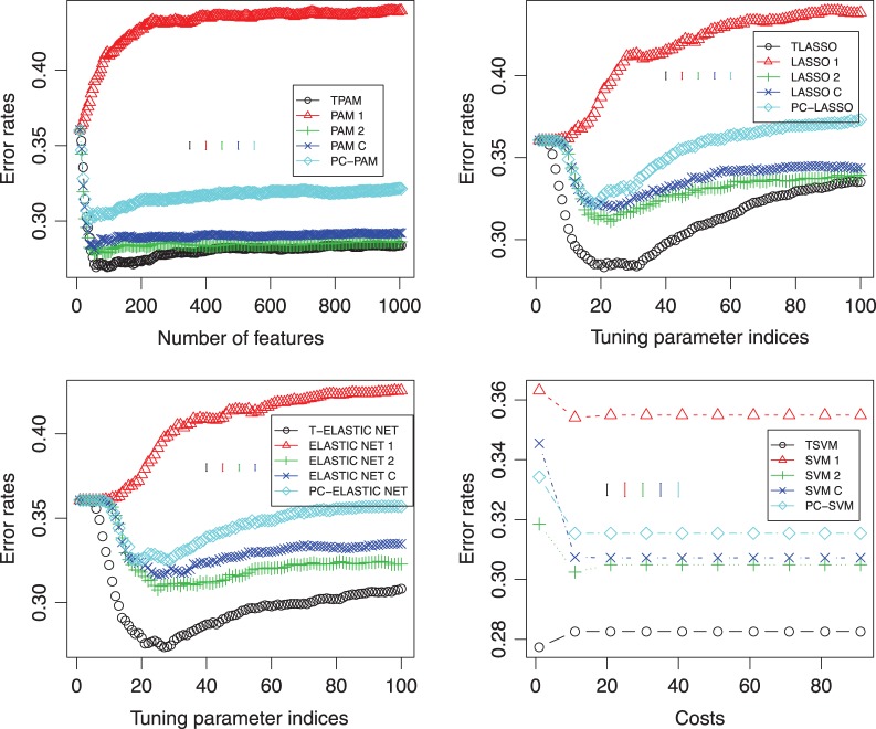
Fig. 4.
Classification performances using different methods at the second stage of our approach as well as using different methods directly on the burn patients’ data. Top-left: TPAM, PAM, and PC-PAM; top-right: TLASSO, LASSO, and PC-LASSO; bottom-left: T-ELASTIC NET, ELASTIC NET, and PC-ELASTIC NET; bottom-right: TSVM, SVM, and PC-SVM. ∘: using the Fisher criterion to obtain the direction of projection at the first stage; △: using the first time point; +: using the second time point; ×: combining the early and middle time points;  : using the first principal component as the direction of projection at the first stage. Y -axis is the error rate on the test data. The X-axis in the top-left panel is the number of features selected in the models. The X-axes in the top-right and bottom-left panels are the indices of the tuning parameter; each index i (i∈{0,…,99}) corresponds to λmax−i(λmax−λmin)/99; λmax is the maximum value of the tuning parameter λ calculated by default by R-package glmnet. λmin=λmaxλmin.ratio and λmin.ratio=0.01, which is the default value of glmnet. The axis in the bottom-right panel is the cost that corresponds to the parameter c in the R-package e1071.

