Figure 12. Shell model for solution of -diffusion problem.

(A) The space is divided in spherical shells of thickness of 20 nm and the channel is localized at the center of this configuration ( Source). The distance of the BK channel to the source is indicated by R. The equations to be solved on this geometry are the diffusion equation and the interaction with the mobile buffer equations 5–7. The mobile buffers Bi are also subject to diffusion. We integrated these equations over the spheres taking N points at the middle of the shells where, and . Integrating gives , where is the calcium concentration at shell j and time n, and similar equations for B_j, the buffer concentrations for each shell. 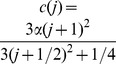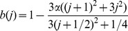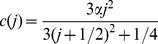The coefficients are,, and and . The diffusion coefficient is 250 m² s⁻¹ [57]. The buffer diffusion constant and rate constants were taken from ref [57] for calmodulin. B. We have solved the matrix equation as explained in the text. The current was converted to Molar s⁻¹ using the equation , where F is Faraday's constant, i is the current and V is the volume of the shell. The source was assumed to open at time 0 and decay with kinetics similar to the T-type channel. (B) Panel B shows the results of the simulation for shells 1(20 nm, open green circles), 3 (60 nm, open green triangles) and 5 (100 nm, open green diamonds). The black traces show the heuristic kinetics used in figure 11 to fit the I component of BK currents. The bars represent 20 M and 20 ms. (C) Same as in B, except that the source was distributed over the first three shells were updated according to the rule 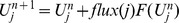where the flux F was (Shell 1), 0.51 (Shell 2) and 0.36 (Shell 3) with . The function F is a saturable function of calcium concentration that represents -dependent inactivation. Panel C shows the results for shells 3 (60 nm, open green circles), 6 (120 nm, open green diamonds), and 15 (300 nm, open red triangles). The black traces show the heuristic kinetics used in figure 11 to fit the I component of BK currents. The bars represent 20 M and 60 ms.