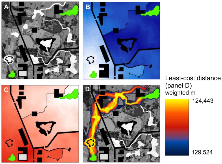
Figure 1. Cost-weighted distance modeling.
(A) Example 3 km×3 km landscape with a pixel size of 3 m (from [15]). Two habitat patches (green) are embedded in a matrix of land cover types with differing resistance to movement. Resistances range from 1 (white) to 100 (dark grey); complete barriers with infinite resistance (e.g., linear features representing roads and highways) are shown in black. (B) Cost-weighted distance (CWD) from leftmost patch, with darker shades representing higher cumulative resistance from the patch. (C) CWD from rightmost patch, with darker shades representing higher cumulative resistance from the patch. (D) Modeled least-cost corridor produced by adding CWD surfaces shown in panels B and C (best 20% of study area shown). The least-costly path (traced in green) has a cumulative least-cost distance (LCD) of 124,443 weighted meters.

