Figure 9.

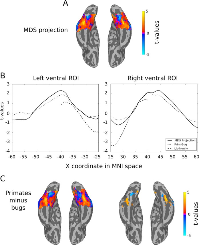
Comparison of the projection of the bugs-to-primates dimension (Fig. 7) to the living–nonliving contrast from Mahon et al. (2009). Using a method described by Mahon et al. (2009), we calculated the medial-to-lateral index for the projected Dimension 1 from the MDS analysis (Fig. 8). A, The colored regions show the extent of the mask used in the analysis, and the colors reflect the unthresholded t values for the group result. The mask we used covers a greater extent of the ventral surface in the medial-to-lateral dimension than that reported by Mahon et al. (2009). While these extra data points played no role in the comparison with the living–nonliving contrast, they illustrate the extent of consistent activity across the ventral surface. B, The medial-to-lateral index for our results and for living–nonliving. The values reported for the living–nonliving contrast were kindly provided to us by Brad Mahon and are also plotted in Mahon et al. (2009; their Fig. 5B, p. 402). The linear fits between our data and the living–nonliving contrast were highly significant with R² of 0.83 and 0.82 for the left and right ROIs, respectively. C, For comparison, we present the results of the contrast of primates and bugs within the left and right ventral ROIs. The unthresholded contrast on the left shows a nearly identical pattern to that of the Dimension 1 projection, which is also reflected by the medial-to-lateral index calculated for the primates–bugs contrast (B). On the right, we plot all voxels that pass a statistical threshold (t₍₁₁₎ > 2.2, p < 0.05) for the contrast. Blue voxels reveal bilateral medial regions in which the activity for bugs was greater than that for primates; warm-colored voxels reveal bilateral regions in the lateral fusiform in which activity was greater for primates.