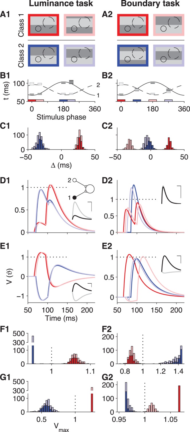
Figure 4. Mechanisms of spike-latency-based neuronal computing.

Illustration of sample tempotrons that solve the luminance (left) or the boundary (right) task. Each tempotron receives inputs from only two RGCs, and only their first spikes are processed. (A) The four grating stimuli that define each task and the relative locations of the two recorded RGC receptive fields. Solid line: Cell 1; dashed line: Cell 2. (B) Latency tuning of the two RGCs under the eight gratings. Lines show fitted cosine tuning curves. Colored horizontal bars highlight the spatial phases of the four stimuli used in each task, color-coded as in (A). For each of these stimuli, boxes depict the mean ±1 SD of the measured first-spike latency. (C) Histograms of the differential latencies  of the two RGCs during the four task-relevant stimuli, color-coded as in (A). (D) Sample voltage traces of a tempotron that solves the task, color-coded according to the four stimuli. The input spike times of this example represent the median differential latencies observed experimentally. Horizontal dotted line depicts the spike threshold. Inset: The minimal readout circuit with two RGCs connected to one postsynaptic neuron. Traces show the PSPs of cell 1 (black) and cell 2 (gray) that underlie the solution shown in the main panel. Scale bars depict 20 ms in the x-direction and half of the spike threshold in the y-direction. In these implementations, both afferents are excitatory. D1:
  , D2:
, D2:  . (E) Like (D), but in these solutions, one afferent is excitatory and the other inhibitory. E1:
  , E2:
, E2:  . Note that the solution in (E2) encodes the identity of the stimulus within the target class by the latency of the output spike: While early responses signal the dark red stimulus, later responses signal the light red stimulus. The membrane time constants in (D) and (E) were chosen to minimize the generalization errors for the sample distributions of (C) in the investigation of threshold noise (Materials and Methods). (F) Histogram of the peak voltage of the tempotron in (D) for all experimental trials, color-coded by stimulus as in (A). Note that the target and null stimuli are well separated on either side of the threshold (dotted vertical line). (G) Like (F), but for the solutions in (E).
